In Part 1 of this series, we briefly touched upon the various design considerations to be made when architecting the Data Lake. We saw how considerations on partitioning, data formats, and schema evolutions are instrumental in making the data accessible in an efficient and performant manner to end-users. We also stepped through a simulation of implementing ingestion to the Data Lake using mature Open Source tools on Qubole. In this part, we deep dive into the design considerations and discuss recommended strategies and experiences from the field.
Mutable and Immutable Data
What is Immutable data?
There are two aspects of immutability in the big data world:
- Storage Systems: HDFS and HDFS compliant storage systems like S3, GCS, etc. store files as immutable. These files cannot be updated with random writes.
- Nature of datasets: Real-world datasets like logs, clickstream data, and IoT event data are immutable. They are facts that cannot be changed.
What is Mutable data?
There are some data sets that change very often. For example – RDBMS transactional data (User-level information, Product details, etc.).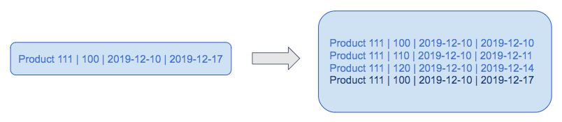
Here, the product with id 111 has been modified three times in one week. This duration could easily be in the order of minutes or years.
Design Consideration: Partitioning and Bucketing Strategy
Partitioning- Partitioning is a way of dividing a table into related parts based on the values of particular columns like date, city, and department. Each table in Hive can have one or more partition keys to identify a particular partition. Big Data engines like Spark, Hive, and Presto can use partitions to limit queries on slices of the data and hence get a performance boost.
- To decide on the partition column, it is imperative to understand the usage pattern. For example, if you know that most of your queries will be using a city level filter in their queries or jobs then partition the data by city column.
- In general, it is recommended to partition your data based on a created-at timestamp
- Overall, data size matters as well. For example, if the data’s total size is a few MBs, then partitioning will not be required because it’ll lead to classic too many small-files problems in big data. And if the data is huge, let’s say in hundreds of GBs or TBs, then multiple partition hierarchies can be used. For example, date=yyyy-mm-dd/hour=hr/ which helps in less data scanning based on the query’s filter criteria.
- If the incoming data doesn’t have the created-at field it would be great to add it to your ingestion pipeline
Bucketing – Partitions are subdivided into buckets based on the hash function of a column in the table to give extra structure to the data that may be used for more efficient queries.
- Join queries get a performance boost if both tables have similar bucketing strategies.
- Ensure that data is distributed evenly with the bucketing strategy.
Let’s see an example of designing the partitioning and bucketing strategy:
Approach 1: Extremely Granular Partitions
Suppose we implement the following partitioning strategy: advertiser_id/year/month/day/hour.
This will store data for each advertiser in a separate path. Further, it will divide the data on an hourly basis. Theoretically, this might seem a good design in keeping with RDBMS-like indexing strategies.
However, our table statistics show:
- 200 unique advertiser_id values
- Five years of data
Hence, with this design scheme, we end up with
- 200 * 5 * 365 * 24 = 8,760,000 partitions
- One, small file per partition
Approach 2: Coarse granularity with query pattern considerations
Learning from the previous approach, we can implement the following strategy:
- Partitioning strategy: year/month/day
- Bucketing strategy: advertiser_id
Now, we will end up with
- 5 * 365 = 1825 partitions
- 200 files per partition
- Optimally sized files per partition
Design Consideration: Change Data Capture
Data is not static. Once the initial (or historical) load is completed, a Change Data Capture (CDC) pipeline should be in place to synchronize change data or delta with your initial load.
In Part 1 of the series, we did a hands-on exercise in Change Data Capture. Further, in the previous section, we discussed the partitioning and bucketing strategy for the data. The delta that we capture can be pertinent to the partitions generated for the historical data or can belong to entirely new partitions.
Hence, it becomes tricky to decide what data sets need to be updated.
For example, if the table has 1000 partitions and you want to refresh everything every hour. This is a costly operation that will require a lot of computing resources.
Based on our experience in the field, here are some recommendations for designing the CDC pipeline:
- Append-only data
- Data arrives and needs to be written to the appropriate partition.
- The INSERT INTO statements in Hive/Spark can help write into static partitions.
- Upserts
- DO NOT try to update all the partitions.
- Evaluate the use-cases: For example, if most use cases demand the latest records of the last three months.
- Here, update only those many partitions every hour and the rest can be updated by a daily job.
Another widely used approach is:
- Create a delta table for the current day data
- Append the incoming data to this table irrespective of UPSERTS or Appends.
- Create a logical View joining the delta table and history table
- This logical view will serve as a consistent, updated VIEW of the data for the end-users.
Design Consideration: Concurrent Reads and Writes
As we saw previously, files written to the Data lake tables are immutable due to the nature of Cloud Storage and HDFS systems. Further, we saw how to add data to the tables using bulk loads and change data capture. Further, other activities on the Data Lake will also perform read or write operations on tables, and often, the same table partition will be used by different users for reading and writing – simultaneously.
Updates to partitions are handled by INSERT OVERWRITE operations on the whole partition. This deletes the old files and writes new ones.
This causes a few problems:
- Queries reading from the existing partition location may fail if the files read by them are deleted by an INSERT OVERWRITE query.
- INSERT OVERWRITE writes directly to the partition path. So for some time, there will be old and new files present in the partition path, and any query on this partition at this time will read redundant data leading to wrong results
- Deletions happen in batches of files, an overlapping read while deletions are going on a can:
- Get a list of new files and some old files and fail while reading old files in a worker process due to the FileNotFound exception
- Get a list of new files and some old files and read the old data as well due to Eventual Consistency and end up with wrong results
To solve these issues, we can avoid writing to the same location from which other users read it. Here is an approach to achieve this:
Requirement
Update the sales_data_history table with yesterday and today’s delta data.
Assumption
The current date is 2019-10-30, and we are running this job in the middle of the day. And there is an empty table sales_data_history_temp which has the same schema as sales_data_history.
Tables
- sales_data_history: Historical sales data partitioned by day.
- sales_data_delta: New and Updated records for 29th and 30th
- sales_data_history_temp: Temporary table for storing the intermediate output
Step 1
Let us update the temporary table with the delta and history data.
The following SQL:
- Takes all the delta records from sales_data_delta
- Takes the latest couple of partitions from history i.e. 29th and 30th.
- De-duplicates the records with the same IDs to handle UPSERTS and INSERT new records as is.
SET hive.exec.dynamic.partition=true;
SET hive.exec.dynamic.partition.mode=nonstrict;INSERT OVERWRITE TABLE sales_data_history_temp PARTITION (day)
SELECT id,
region,
country,
item_type,
sales_channel,
order_priority,
order_date,
order_id,
ship_date,
units_sold,
unit_price,
unit_cost,
total_revenue,
total_cost,
total_profit,
created_at,
updated_at,
from_unixtime(unix_timestamp(created_at,'MM/dd/yyyy'),'yyyy-MM-dd') # partition column
FROM
(
SELECT RANK() OVER w AS rank, ROW_NUMBER() OVER w AS row_num, t1.*
FROM
(
SELECT * FROM sales_data_history WHERE day = '2019-10-29' or date = '2019-10-30'
UNION ALL
SELECT *, from_unixtime(unix_timestamp(created_at,'MM/dd/yyyy'),'yyyy-MM-dd') FROM sales_data_delta;
) t1
WINDOW w AS (PARTITION BY t1.id ORDER BY updated_at DESC)
) t
WHERE rank = 1 and row_num = 1;
After execution of this query, the sales_data_history_temp table would have only two partitions:
s3://<bucket>/data/sales_data_history_temp/day=2019-10-29
s3://<bucket>/data/sales_data_history_temp/day=2019-10-30
Step 2
Now, set these two locations as the latest partitions for our main history table sales_data_history:
ALTER TABLE sales_data_history PARTITION (day='2019-10-29')
SET LOCATION 's3://<bucket>/data/sales_data_history_temp/day=2019-10-29';ALTER TABLE sales_data_history PARTITION (day='2019-10-30')
SET LOCATION 's3://<bucket>/data/sales_data_history_temp/day=2019-10-30';
Design Consideration: Small files and Skewed Partitions
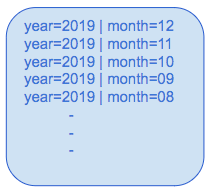
During the continuous data ingestion process, most of the records will belong to the recent partitions. Hence, they will be skewed. For example, the majority of the records belong to the 12th month:
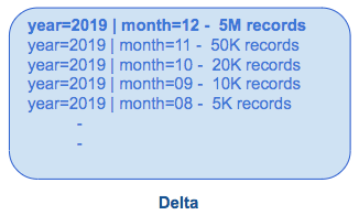
Here, the INSERT OVERWRITE will be slower (based on the query) as most of our records are for the same partition. Based on our field experience, here are some recommendations to handle this:
- DISTRIBUTED BY: This clause reshuffles your data to avoid skewness while writing.
- Handle the skewed partition separately.
- Engine Tuning: Adjust the Number of Reducers(Hive) or the Number of Shuffle Partitions(Spark) according to the requirement.
An alternative approach is to optimize the data in the storage itself i.e. merge small files:
Design Consideration: Schema evolution
It allows users to easily change a table’s current schema to accommodate changing data over time to handle new business use cases. It’s most commonly used when performing an append or overwrite operation, to automatically adapt the schema to include one or more new columns. There are multiple file formats available in a modern data lake, and some major ones are – CSV, JSON, Avro, Parquet, and ORC. These formats have some behavioral differences and are mentioned in the below table.
If you have a Metadata layer, for SQL (Hive, Presto, Spark-SQL, etc.), on top of the data, then you can decide the file format based on the schema operations required.
| Generic schema operations | |||||||
| Rename column | Add column | Remove column | Reorder | Data type change | |||
| At the beginning/Middle | At the end | ||||||
| CSV/TSV | Y | N | Y | N | N | Y | |
| JSON | N | Y | Y | Y | Y | Y | |
| Avro | N | Y | Y | Y | Y | Y | |
| ORC | Read by index | Y | N | Y | N | N | Y |
| Read by name | N | Y | Y | Y | Y | Y | |
| Parquet | Read by index | Y | N | Y | N | N | Y |
| Read by name | N | Y | Y | Y | Y | Y | |
Additionally, in Spark (Python, Scala, R), by including the mergeSchema option in your query, any columns that are present in the DataFrame but not in the target table are automatically added to the end of the schema as part of a write transaction. Nested fields can also be added, and these fields will get added to the end of their respective struct columns as well. Here, add-column and data-type-change to upcast schema changes are eligible for schema evolution during table appends or overwrites.
# Add the mergeSchema option

dataFrame.write.format("parquet") \

.option("mergeSchema", "true") \

.mode("append") \

.save(MY_OUTPUT_PATH)
Other changes, which are not eligible for schema evolution, require that the schema and data be overwritten by the option overwriteSchema. Here, add-column, remove-column, data-type-change, and rename-column operations could be supported.
Although there are many file formats available with the different features set, few recommendations have been made to have a seamless experience.
- Avoid adding a column in the middle of the schema
- Avoid changing the data types of the columns. If required, then make sure that the changes are backward compatible. For example, string type columns should not be converted into Numeric data types because they may break at query execution time.
- Avoid removing columns unless you are entirely overwriting the data
- Don’t use the column name as a partition column if it is already used in the file schema
- Try to use lower-case column names all across to ignore case sensitivity issues in some processing engines