This post covers the use of Qubole, Zeppelin, PySpark, and H2O PySparkling to develop a sentiment analysis model capable of providing real-time alerts on customer product reviews. In particular, this model allows users to monitor any natural language text (such as social media posts or Amazon reviews) and receive alerts when customers post extremely nice (high sentiment) or extremely negative (low sentiment) comments about their products.
In addition to introducing the frameworks used, we will also discuss the concepts of embedding spaces, sentiment analysis, deep neural networks, grid search, stop words, data visualization, and data preparation.
Setting Up the Environment
Our first task is to set up our environment inside Qubole. We create a notebook in four easy steps:
- Click New.
- Provide a name.
- Select the appropriate language and version number. For this particular example, we choose PySpark (v2.1.1) given its ease of handling large data sets and access to the H2O Pysparkling library (v2.1.23).
- Update bootstrap file to allow access to H2O’s Sparkling Water framework.
Once the environment is set up in Qubole, the next step in building a sentiment analysis model is to collect labeled, unstructured text data (known sentiment scores) from the reviews. In our case, we choose to use Amazon’s Product Reviews. Amazon hosts a massive data set of product reviews on their Simple Storage Service (S3) that is free to access and use. The data is available in Parquet format or tab-separated format.
The overall process of using these reviews to generate and use a semantic analysis engine based on a deep neural network model is shown in the Figure below. Our steps will include:
Ingesting the data into a PySpark DataFrame
- Exploring and visualizing the data to better understand available information
- Cleaning the data to ensure we have good content going into the model learning process
- Learning a Word2Vec embedding space based on the unstructured content of the reviews
Splitting the data into a training set and a test set
Performing a grid search to optimize the parameters used in our deep learning model
- Training the deep learning model
- Using the trained model to predict the star ratings of product reviews
Converting the model into a sentiment analysis tool that alerts you to social media-based product reviews and comments
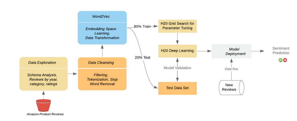
Figure 1: To process these reviews, we need to explore the source data to: understand the schema and design the best approach to utilize the data, cleanse the data to prepare it for use in the model training process, learn a Word2Vec embedding space to optimize the accuracy and extensibility of the final model, create the deep learning model based on semantic understanding, and deploy the system to analyze new reviews and provide sentiment predictions.
Step 0: Ingestion of Review Data
Before we can start, we first need to access and ingest the data from its location in an S3 datastore and put it into a PySpark DataFrame (for more information, see this programming guide and select Python tabs).
%pyspark
import h2o
from h2o.estimators.word2vec import H2OWord2vecEstimator
from h2o.estimators.gbm import H2OGradientBoostingEstimator
from h2o.estimators.deeplearning import H2OAutoEncoderEstimator, H2ODeepLearningEstimator
from pysparkling import *
from nltk.corpus import stopwords

hc = H2OContext.getOrCreate(sc)
data_file = "s3://amazon-reviews-pds/tsv/"
data = spark.read.parquet("s3://amazon-reviews-pds/parquet/")
Step 1: Data Exploration
Now that we have the data in the system, we want to better understand what information the data contains and how we can best use it to our advantage. To achieve this goal, we will do a series of visualizations of the data starting with a simple count of the number of reviews in the data set.
We find that we have more than enough reviews (over 160 million) to build a solid sentiment analysis model.
Total Number of Reviews in the Dataset:
160796570
Next, let’s take a look at the schema of the data (or what attributes are available for each of the reviews). This goal can be achieved by asking for a list of the column names on the data frame. The result is a list of the attributes available to us for each review. These include:
‘marketplace’, ‘customer_id’, ‘review_id’, ‘product_id’, ‘product_parent’, ‘product_title’, ‘star_rating’, ‘helpful_votes’, ‘total_votes’, ‘vine’, ‘verified_purchase’, ‘review_headline’, ‘review_body’, ‘review_date’, ‘year’, ‘product_category’
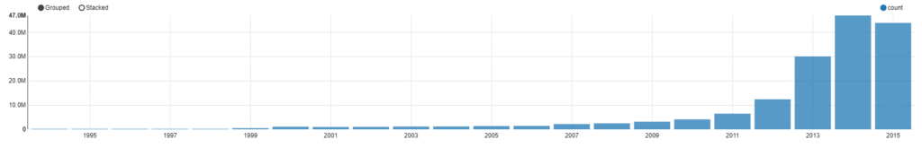
Looking through these column names, we notice that it includes the year of the review and decide to see how many reviews per year are in the data set. The result shows us there are few reviews in the early years (including one from 1970, which is almost certainly a null date that defaulted to the Epoch) and the number grows until 2015, which is the final year of the data set.
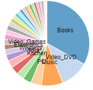
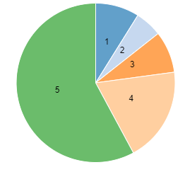
Given the overall size of the data set, we decide to work with a more manageable quantity and choose a specific year to analyze: 2009. This filtering leaves us with just over three million reviews. We then want to see what categories are covered by the data set and the relative number of reviews for each of these categories.
To accomplish this, we group the data by the “product_category” attribute, count the number of reviews in each of the categories, and sort them by the total number. We then plot it as a pie graph (shown below). There are a total of 42 categories ranging from the most popular to review – books – and going to the least popular to review – gift cards.
We are then interested in the relative number of reviews that received the possible range of star ratings (1-5). Similar to above, we group the reviews by the attribute of interest (“star_rating”), count them, and sort them from most popular to least popular. The resulting pie chart shows that positive reviews are significantly more common than bad reviews, with a two-star rating being the least popular score.
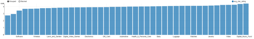
Next, we want to better understand the relationship between product category and rating. Do certain categories have higher or lower average ratings? As shown in the figure below, the highest average rated categories are digital music purchases (4.44), music (4.375), and groceries (4.269). The lowest average rated categories are digital software (2.76), appliances (2.961), and software (3.446).
We decide to further filter the data down to a specific category, as people might use different words to express positivity or negativity across different categories. For example, saying “the fruit arrived perfectly ripe” is likely a positive remark, while saying “my new pair of shoes smelled ripe when they arrived” is almost certainly a negative remark.
After choosing the sports category for the year 2009, we want to understand the top words for each star rating. First, we select the attribute that contains the unstructured text content of the review — the “review_body” — and split the text into individual words through a process called tokenization. Fortunately, PySpark has a simple tokenizer capability called RegexTokenizer that splits unstructured text via a provided regular expression.
In our case, we want to split the text by white spaces and use the simple pattern “\\W+” to keep any number of consecutive letters together within the same token. This pattern drops numbers, punctuation, and spaces. In addition, we choose to only keep words with at least three characters. Using this tokenizer, the sentence “I hit the ball a hundred yards farther with this new club” would be split into 10 tokens (hit, the ball, hundred, yards, further, with, this, new, club). We then filter the data to include ratings with the specified star count (five in this case) and run the reviews through the tokenizer.
Once tokenized, we want to remove common words that convey minimal meaning such as “the” and “and”. To accomplish this goal, we use another helpful PySpark feature, StopWordsRemover. This function simply removes the stop words from the input column (“tokenized_words”) and places the output in a separate column (“word_tokens”).
Finally, now that we have a collection of all of the words used in the five-star reviews, we can group, count, and sort the results from highest to lowest. The list below shows the top ten words used in five-star reviews in the sports category in 2009. The fact that these are all positive sentiment words means that a model trained on this data would likely provide the desired functionality.
| Word | Count |
| great | 14585 |
| one | 11846 |
| use | 9210 |
| good | 8760 |
| well | 8547 |
| like | 8447 |
| would | 7798 |
| get | 7511 |
| product | 6845 |
| easy | 6094 |
%pyspark
# Size of the Review Tables (Row Count)
print("Total Number of Reviews in the Dataset:")
data.count()
%pyspark
# Print Schema
print("Dataset Schema (Column Names)")
data.columns%pyspark
# Plot of # of Reviews by Year
z.show(data.groupBy("year").count().sort("year"))%pyspark
year = 2009
print("Filtered Number of Reviews in {0}:".format(year))
filtered_data_year = data.filter(data.year == year)
filtered_data_year.count()%pyspark
z.show(filtered_data_year.groupBy("product_category").count().sort("count", ascending=False))%pyspark
z.show(filtered_data_year.groupBy("star_rating").count().sort("star_rating", ascending=False))%pyspark
from pyspark.sql import functions as F
# Avg star_rating by Product_Category
z.show(filtered_data_year.groupBy("product_category").agg(F.mean("star_rating").alias("avg_star_rating")).orderBy("avg_star_rating"))%pyspark category = "Sports" filtered_data_year_category = filtered_data_year.filter(data.product_category == category)
%pyspark
stars = 5
from pyspark.ml.feature import RegexTokenizer, StopWordsRemover
import pyspark.sql.functions as f
tokenizer = RegexTokenizer(inputCol='review_body', outputCol = 'tokenized_words', pattern="\\W+", minTokenLength = 3)
filter_star_rating = filtered_data_year_category.filter(filtered_data_year_category.star_rating == stars)
tokenized_words = tokenizer.transform(filter_star_rating)
remover = StopWordsRemover(inputCol='tokenized_words', outputCol = 'word_tokens')
clean_tokens = remover.transform(tokenized_words)
word_counts = clean_tokens.withColumn('word', f.explode(f.col('word_tokens'))).groupBy('word').count().sort('count', ascending=False)
z.show(word_counts)
Step 2: Data Cleansing and Preparation
Now that we have a good data set and understand the different attributes available to us, we can proceed to build the actual sentiment analysis model. Since we are planning on building the model in the H2O framework, our first step is to convert the PySpark DataFrame into an H2O DataFrame. Counting the number of rows we will use to build the model, we find we have over sixty thousand reviews. While we would likely get a more accurate model by using all of the sports category reviews across all years, for this demonstration we’ll stick with the sixty thousand reviews for speed considerations.
To show the full capabilities of H2O, we will now repeat a few steps from above including tokenization and stopword removal. First, we load a collection of stopwords from NLTK. (NLTK provides a collection of useful data sources for natural language processing at https://www.nltk.org/nltk_data) We also define the function “tokenize” that takes in the review and, much like before, splits it into individual words while removing stopwords.
We then call the tokenize function on the “review_body” attribute of each review.
%pyspark
dataH2 = hc.as_h2o_frame(filtered_data_year_category)
print("Number of Reviews Being Analyzed in H2O:")
dataH2.nrow
%pyspark
STOP_WORDS = stopwords.words("english")
def tokenize(sentences, stop_word = STOP_WORDS):
tokenized = sentences.tokenize("\\W+")
tokenized_lower = tokenized.tolower()
tokenized_filtered = tokenized_lower[(tokenized_lower.nchar() >=2) | (tokenized_lower.isna()),:]
tokenized_words = tokenized_filtered[tokenized_filtered.grep("[0-9]", invert=True, output_logical=True),:]
tokenized_words = tokenized_words[(tokenized_words.isna()) | (~ tokenized_words.isin(STOP_WORDS)),:]
return tokenized_words%pyspark dataH2.nrow words = tokenize(dataH2['review_body'
Step 3: Learning an Embedding Space
Once we have the tokenized words, our next step is to train a semantic embedding space. Embedding spaces help solve the matrix sparsity issue within the natural language processing domain. Historically, each word has been treated as a different value of the model’s input vector. This results in a very long input vector with a single 1 among numerous 0s. The resulting model often becomes overfit to the training data.
With embedding spaces, each word becomes a dense vector of set length with values ranging from 0 to 1. This vector represents the semantic usage of the specific word instance provided in the training data. As a result, semantically similar words will be near each other within the embedding space and will allow the NLP model to share information across various words of a similar nature. One of the best parts about embedding spaces is the lack of a need for labeled training data. You can simply provide a large amount of unstructured text and the system will automatically learn the embedding space. There are many ways of building embedding spaces, but we will use the simple approach of using H2O’s built-in Word2VecEstimator.
Of note, however, is that the data used to train the model should be from the same domain as the data you plan on analyzing. The use of the same domain will avoid issues with different lexicons being used and different meanings of the same word occurring in different ways across domains.
To demonstrate the use of an embedding space, we will show semantically similar words for “wonderful”. Given H20’s simple API, this requires a simple function call on the model “word2vec.find_synonyms” with the variables being the source word and the number of similar words you would like returned. As you can see in the table below, all of the listed words could easily replace “wonderful” in a sentence with little change in meaning. Of note, the misspelling of excellant (sic) is included in the list but would never show up in a standard thesaurus. This is part of the power of embedding spaces. Due to the lack of a need for labeled training data or human input, the system is able to understand the semantic behind words even if they don’t appear in a dictionary.
| Word | Similarity Score |
| great | 0.759 |
| fantastic | 0.746 |
| excellent | 0.697 |
| terrific | 0.692 |
| love | 0.656 |
| pleasure | 0.638 |
| outstanding | 0.620 |
| excellant | 0.613 |
| appreciated | 0.608 |
| awesome | 0.600 |
Now that we have an embedding space, we need to put it to work transforming the individual words in each review into a vector. We do this with a simple call to “transform” that converts each word in a review to a vector and then averages the resultant vectors to provide a single vector representing the entire review comment.
%pyspark
word2vec = H2OWord2vecEstimator(sent_sample_rate = 0.0, epochs = 2)
word2vec.train(training_frame=words)
%pyspark
w = "wonderful"
print("Synonyms for " + w)
word2vec.find_synonyms(w, count = 10)
%pyspark review_vectors = word2vec.transform(words, aggregate_method="AVERAGE")
Step 4: Deep Learning Model Generation
Now that we have a more semantic model of our reviews, we are ready to build a predictive model that will take a new comment about a product and produce a prediction of the star rating associated with the comment. Our first step is to continue cleansing the data, remove all null valued reviews, and split the data into two sections that will later be used as a training set and a test set.
Our next step is to learn the best parameters for the deep neural network that we will use as our predictive model. In general, you would provide a wide range of possible values for each of the parameters and see which ones provide the best Log Loss score, and then use those parameters to tune a final model. However, to keep things simple, we only consider a handful of potential values for the three parameters we will use in specifying our H20 deep learning model: the number of layers, the number of nodes in each layer, and the L1 Regularization parameter. For the width and depth of the model, we allow for five different configurations:
- A 4-layer model with the input layer, a 17 node layer, a 32 node layer, and the output layer
- A 4-layer model with the input layer, an 8 node layer, a 19 node layer, and the output layer
- A 5-layer model with the input layer, a 32 node layer, a 16 node layer, an 8 node layer, and the output layer
- A 6-layer model with the input layer, four layers of 100 nodes each, and the output layer
- A 6-layer model with the input layer, four layers of 10 nodes each, and the output layer
For the L1 regularization parameter, we allow the value to range from 1e-6 to 1e-3.
We then use H20’s convenient function H2OGridSearch to set up the grid search and select the H2ODeepLearningEstimator as the model type for analysis. (Check out this H2O documentation for more information on H2OGrid Search.)
Once completed, we want to see the results of the grid search. We find that the model with the lowest Log Loss score is model 0, which uses a 5-layer deep neural network with an L1 regularization parameter of 3.85e-4.
| Model # | Hidden Layers | L1 Parameter | Log Loss Score |
| 0 | 32, 16, 8 | 3.85E-4 | 0.985 |
| 1 | 32, 16, 8 | 2.0E-5 | 0.992 |
| 2 | 100, 100, 100, 100 | 3.55E-4 | 1.003 |
| 3 | 17, 32 | 7.9E-4 | 1.004 |
Now that we have the best parameters for the model, we will define the model with these parameters and then train it on the complete data set. We will use the first 80 percent of the data as training and the second 20 percent for validation. Once trained, we print out the model performance scores (shown below) to see how accurate the overall model is at predicting the star rating. As you can see, the model isn’t very accurate and has trouble predicting scores of 2, 3, and 4. If we wanted to improve this accuracy, the best approach would be to go back and even out the number of training samples for each of the rating values, because they are heavily skewed to 5s and 1s right now.
Model Metrics Multinomial: Deep Learning
** Reported on validation data. **
MSE: 0.348988435508
RMSE: 0.590752431656
LogLoss: 1.01519510962
Mean Per-Class Error: 0.615470556769
| Predicted | |||||||
| Actual | 1 | 2 | 3 | 4 | 5 | Error Rate | |
| 1 | 65 | 0 | 6 | 4 | 22 | 0.329897 | 32/97 |
| 2 | 17 | 1 | 12 | 12 | 22 | 0.984375 | 63/64 |
| 3 | 12 | 0 | 11 | 15 | 40 | 0.858974 | 67/78 |
| 4 | 7 | 0 | 15 | 47 | 162 | 0.796537 | 184/231 |
| 5 | 14 | 1 | 7 | 32 | 448 | 0.10757 | 54/502 |
| 115 | 2 | 51 | 110 | 694 | 0.411523 | 400/972 | |
With the model trained, it is now time to start making predictions on new product reviews. To do so, we need a function that will take any unstructured text comment and return a predicted score.
Now, we can send it any text and get back a result. As you can see below, the model predicts the star rating of the phrase “This is the best product in the world!” as a 5-star review.
Checking prediction for the following review:
This is the best product in the world!
| Prediction | Prob(1) | Prob(2) | Prob(3) | Prob(4) | Prob(5) |
| 5 | 9.55421e-05 | 6.21569e-05 | 0.00143779 | 0.0147145 | 0.98369 |
%pyspark
valid_reviews = ~ review_vectors["C1"].isna()
fulldata = dataH2[valid_reviews, :].cbind(review_vectors[valid_reviews,:])
fulldata[:,6] = fulldata[:,6].asfactor()
data_split = fulldata.split_frame(ratios=[0.8])
%pyspark
hidden_opt = [[17,32],[8,19],[32,16,8],[100,100,100,100],[10,10,10,10]]
l1_opt = [s/1e6 for s in range(1,1001)]
hyper_parameters = {"hidden":hidden_opt, "l1":l1_opt}
search_criteria = {"strategy":"RandomDiscrete", "max_models":10, "max_runtime_secs":100, "seed":123456}
from h2o.grid.grid_search import H2OGridSearch
model_grid = H2OGridSearch(H2ODeepLearningEstimator, hyper_params=hyper_parameters, search_criteria=search_criteria)
model_grid.train(x=review_vectors.names,
    y="star_rating",
    distribution="multinomial",
    epochs = 1000,
    training_frame = data_split[0],
    validation_frame = data_split[1],
    score_interval=2,
    stopping_rounds=3,
    stopping_tolerance=0.05,
    stopping_metric="misclassification")
%pyspark model_grid
%pyspark
dl_model_v2 = H2ODeepLearningEstimator(
    model_id = "model_v2",
    distribution = "multinomial",
    hidden = [10, 10, 10, 10],
    epochs = 1000,
    score_validation_samples = 1000,
    score_interval = 2,
    stopping_rounds = 3,
    stopping_metric = "misclassification",
    stopping_tolerance = 0.05,
    nfolds=5)
dl_model_v2.train(x=review_vectors.names,
    y="star_rating",
    training_frame = data_split[0],
    validation_frame = data_split[1])
dl_model_v2.model_performance(valid=True)
Step 5: Sentiment Analysis
You can now use the learned model to automatically determine the sentiment of social media discussions around your product.
For example, if you are monitoring Twitter and a tweet comes in about your product, you can score the social sentiment about your product and be alerted if the sentiment is above or below a threshold. This will allow you to react significantly faster and put out fires or reward key influencers to improve your overall brand value.
Running any comment about a product (e.g. a tweet) through the trained deep learning model will provide a sentiment prediction. For example, the comment “These are the worst. They fell apart after a week of wearing them.” results in the system alerting the user that a Very Negative Sentiment comment was just posted. With this information in hand, the user can follow up with the poster and see if the issue can be resolved (such as sending a refund or a replacement pair). This type of rapid reaction to social media can head off major issues before they become issues.
Analyzing the following tweet:
These cleats are the worst. They fell apart after a week of wearing them.
Very Negative Sentiment – Follow up and discuss the issue with the user.
Let’s try one more product comment: “These are the best cleats ever. I scored three goals in my first game wearing them.” The predicted sentiment for this comment is Very Positive. In this case, the user might want to follow up with the reviewer and offer a reward for the positive review to help bolster their product image.
Analyzing the following tweet:
These are the best cleats ever. I scored three goals in my first game wearing them
Very Positive Sentiment – Follow up and reward the user.
%pyspark
def predict(review, word2vec, prediction_model):
    words = tokenize(h2o.H2OFrame(review).ascharacter())
    review_vec = word2vec.transform(words, aggregate_method="AVERAGE")
    print(prediction_model.predict(test_data=review_vec))
%pyspark
review = "This is the best product in the world!"
print("Checking prediction for the following review:")
print(review)
print(predict([review], word2vec, dl_model_v2))%pyspark
def getSentiment(review, word2vec, prediction_model):
words = tokenize(h2o.H2OFrame(review).ascharacter())
review_vec = word2vec.transform(words, aggregate_method="AVERAGE")
prediction = prediction_model.predict(test_data=review_vec)
if prediction[0, 0] == '1':
print("Very Negative Sentiment - Follow up and discuss the issue with the user.")
elif prediction[0, 0] == '2':
print("Negative Sentiment")
elif prediction[0, 0] == '3':
print("Neutral Sentiment")
elif prediction[0, 0] == '4':
print("Positive Sentiment")
elif prediction[0, 0] == '5':
print("Very Positive Sentiment - Follow up and reward the user.")%pyspark
tweet = "These cleats are the worst. They fell apart after a week of wearing them."
print("Analyzing the following tweet:")
print(tweet)
prediction = getSentiment([tweet], word2vec, dl_model_v%pyspark
tweet2 = "These are the best cleats ever. I scored three goals in my first game wearing them"
print("Analyzing the following tweet:")
print(tweet2)
prediction = getSentiment([tweet2], word2vec, dl_model_v2)Conclusion
In summary, this post shows how to use the combination of Qubole, Zeppelin, PySpark, and H2O’s Pysparking to train a sentiment analysis model based on a collection of Amazon Product Reviews. Qubole provides the architecture and rapid development and deployment environment to get the system up and running in no time. Zeppelin provides a way to quickly visualize the data. H2O Pysparkling allows the training and deployment of machine learning models in a simple, convenient package — providing a low entry bar for using machine learning to solve everyday problems. The developed model can now be used to provide a market monitoring analyst with a real-time understanding of the sentiment being expressed by the public about their product and/or brand.
You can also download the entire notebook for this example.
For additional information on these topics, consider visiting the following sites:
H2O’s Pysparkling – https://docs.h2o.ai/sparkling-water/2.1/latest-stable/doc/pysparkling.html
H2O Word2Vec – https://docs.h2o.ai/h2o/latest-stable/h2o-docs/data-science/word2vec.html
H2O Deep Learning – https://docs.h2o.ai/h2o/latest-stable/h2o-docs/data-science/deep-learning.html
PySpark Data Frames – https://spark.apache.org/docs/2.1.1/sql-programming-guide.html
PySpark – https://spark.apache.org/docs/latest/api/python/index.html
Zeppelin – https://zeppelin.apache.org/