Have you ever wondered why you receive personalized promotions and offers in the mail from various retail and telecom giants? Many of these promotions are a direct result of personalized data science models developed by corporations to figure out which customers are at risk for attrition. For those at risk, the companies create and deliver unique offers based on each individual’s ‘customer profile’ in an attempt to retain their business.
In this article, we will explore using a Customer Attrition Predictive Model to build a relatively straightforward ML application using Apache Spark and a reference dataset available as part of the R C50 package, which we will herein refer to as “Telco Customer Churn Data Set.”
A large number of data science projects revolve around binary classification problems like Customer Attrition. There are many classification algorithms such as Logistic Regression, Support Vector Machines (SVM), Decision Trees, Random Forest Trees, Gradient Boosting, XGBoost, etc. However, there is no single master algorithm that is a clear winner every time. More often than not, the winning algorithm depends on the dataset itself. In this context, the approach to solving classification problems involves training, testing, and comparing multiple algorithms.
For the scope of this article, we will focus solely on XGBoost (a distributed machine learning algorithm) and the Telco Customer Churn Dataset to train and predict Customer Churn using Apache Spark ML pipelines. We will then explore productionizing the trained XGBoost ML pipeline behind a Customer Web Portal to perform real-time scoring of a customer and present tailored offers to preempt customer churn. Through this journey, we will also cover the machine learning portability formats Predictive Model Markup Language (PMML) and Portable Format for Analytics (PFA) for model export. We’ll look at salient features as well as the drawbacks of each, before exploring model deployment and real-time scoring that will deliver continuous business value by making customer retention a reality.
Getting to Know XGBoost, Apache Spark, and Flask
XGBoost is an optimized machine learning algorithm that uses distributed gradient boosting designed to be highly efficient, flexible, and portable. XGBoost provides a parallel tree boosting (also known as GBDT, GBM) that solves many data science problems in a fast and accurate way. XGBoost is a very popular algorithm that has won many data science competitions and challenges at Kaggle and elsewhere.
Apache Spark is an in-memory cluster computing framework originally developed at the University of California, Berkeley’s AMPLab. Spark excels in use cases like continuous applications that require streaming data to be processed, analyzed, and stored. Besides this, Spark is also used widely for Advanced Analytics where Data Science can be done at scale using MLlib’s distributed implementation of several supervised and unsupervised learning algorithms.
Flask is a micro web framework written in Python. It is classified as a microframework because it does not require particular tools or libraries.
About the Reference Data Set:
The Telco Customer Churn dataset contains information corresponding to a single subscriber (customer), as well as whether that subscriber (customer) went on to stop using the service. The dataset presents all the relevant information gathered for each customer when their service was active as 5,000 observations, i.e. subscribers (customers). This is a classic example of a labeled data set, where the churned attribute indicates attrition. In this case, the true value for churn means that the customer has terminated the relationship with the telco and quit using their service. In contrast to the clean dataset, we are using here, the data scientists will put much more work in data wrangling and ensuring data quality(for eg: clean up missing values and anomalies) before the data can be considered as usable for predictive analytics.
Data Ingestion:
The code block below is loading the telco customer churn data file into a data set after some cleansing like filtering out the null rows and transforming/expressing most data types as a numeric value (double).
import org.apache.spark.sql.types.{StructType,StructField,IntegerType,LongType,DoubleType,DateType,StringType}
import java.sql.{Date,Timestamp}
import org.apache.spark.sql.Row
import java.text.{DateFormat,SimpleDateFormat}
import org.apache.spark.ml.feature.ChiSqSelector

val session = org.apache.spark.sql.SparkSession.builder
        .appName("CustomerAttrition")
        .getOrCreate;

case class CustomerChurn(state: String,
account_length: Double,area_code: String,
phone: String, intl_plan: String, voice_mail_plan: String,
number_vmail_messages: Double, total_day_minutes: Double,
total_day_calls: Double, total_day_charge: Double,
total_eve_minutes: Double, total_eve_calls: Double,
total_eve_charge: Double, total_night_minutes: Double,
total_night_calls: Double, total_night_charge: Double,
total_intl_minutes: Double, total_intl_calls: Double,
total_intl_charge: Double,
number_customer_service_calls: Double, churned: String)

val churnsAllDS=spark.read.format("csv")
        .option("header", "false")
        .load("s3://qubole-preddy.us/datasets/telco_churn/churn.all.txt")
        .filter(_.get(0) != null)
        .withColumn("state",$"_c0")
        .withColumn("account_length", $"_c1".cast(DoubleType))
        .withColumn("area_code", $"_c2")
        .withColumn("phone", $"_c3")
        .withColumn("intl_plan",$"_c4")
        .withColumn("voice_mail_plan",$"_c5")
        .withColumn("number_vmail_messages",$"_c6".cast(DoubleType))
        .withColumn("total_day_minutes", $"_c7".cast(DoubleType))
        .withColumn("total_day_calls",$"_c8".cast(DoubleType))
        .withColumn("total_day_charge",$"_c9".cast(DoubleType))
        .withColumn("total_eve_minutes",$"_c10".cast(DoubleType))
        .withColumn("total_eve_calls",$"_c11".cast(DoubleType))
        .withColumn("total_eve_charge",$"_c12".cast(DoubleType))
        .withColumn("total_night_minutes",$"_c13".cast(DoubleType))
        .withColumn("total_night_calls",$"_c14".cast(DoubleType))
        .withColumn("total_night_charge",$"_c15".cast(DoubleType))
        .withColumn("total_intl_minutes",$"_c16".cast(DoubleType))
        .withColumn("total_intl_calls",$"_c17".cast(DoubleType))
        .withColumn("total_intl_charge",$"_c18".cast(DoubleType))
        .withColumn("number_customer_service_calls",$"_c19".cast(DoubleType))
        .withColumn("churned",$"_c20")
Initialize ML Pipeline and Train Model
We are now ready to initialize the machine learning pipeline, which will independently train XGBoostClassifier to be able to predict customer churn on unseen data. Please note that XGBoostClassifier is not natively available in Spark but it integrates well into the Spark ML pipeline API. To use XGBoostClassifier, the following maven dependency “ml.dmlc:xgboost4j-spark:0.80” would need to be supplied. Maven dependencies specified using packages switch in spark-submit and spark-shell gets automatically resolved. The last line of the code block below will let 70% of data available annotated as a train set into the pipeline and roll through all the defined stages including model training.
import ml.dmlc.xgboost4j.scala.spark.XGBoostClassifier
import org.apache.spark.ml.Pipeline
import ml.dmlc.xgboost4j.scala.spark.XGBoostClassifier
import org.apache.spark.ml.feature.VectorAssembler
import org.apache.spark.ml.feature.{OneHotEncoder, StringIndexer}

val XGBoost_pipeline = new Pipeline()

val featureAttributeArray=Array("account_length","intl_plan_indexed",
"voice_mail_plan_indexed","number_vmail_messages","total_day_minutes",
"total_day_calls","total_day_charge",
"total_eve_minutes", "total_eve_calls",
"total_eve_charge","total_night_minutes",
"total_night_calls","total_night_charge",
"total_intl_minutes", "total_intl_calls",
"total_intl_charge","number_customer_service_calls")

val churnIndexer = new StringIndexer().setInputCol("churned").setOutputCol("label")

val indexedChurnDS = churnIndexer.fit(churnsAllDS).transform(churnsAllDS)

val intlPlanIndexer = new StringIndexer().setInputCol("intl_plan").setOutputCol("intl_plan_indexed")

val vMailPlanindexer = new StringIndexer().setInputCol("voice_mail_plan").setOutputCol("voice_mail_plan_indexed")

val vectorAssembler = new VectorAssembler().setInputCols(featureAttributeArray).setOutputCol("features")

val selector = new ChiSqSelector()
      .setNumTopFeatures(12)
      .setFeaturesCol("features")
      .setLabelCol("label")
      .setOutputCol("selectedFeatures")

val xgbParam =Map[String, Any](
           "num_round" -> 5,
           "objective" -> "binary:logistic",
           "nworkers" -> 16,
           "nthreads" -> 4
         )

val xgbClassifier = new XGBoostClassifier(xgbParam).
      setFeaturesCol("selectedFeatures").
      setLabelCol("label")

// Define stages of transformation that will yield a trained Model when the model is fitted using training data.
XGBoost_pipeline.setStages(Array(intlPlanIndexer,vMailPlanindexer,vectorAssembler, selector, xgbClassifier))

// Split the data into training and test sets (30% held out for testing).
val Array(training, test) = churnsAllDS.randomSplit(Array(0.7, 0.3))

val xgBoostModel = XGBoost_pipeline.fit(training)
Model Evaluation:
For binary classification model evaluation, we will use the 30 percent of the data which was set aside and annotated as a test set. Below are a few metrics that help evaluate the model performance.
Accuracy: Accuracy is the most intuitive performance measure, and it is simply a ratio of correctly predicted observations to the total observations. One may think if we have high accuracy then our model is best. Yes, accuracy is a great measure, but only when you have symmetric datasets where values of false positives and false negatives are almost the same.
Precision and Recall: While Recall expresses the ability to find all relevant instances in a dataset, Precision expresses the proportion of the data points our model says were relevant are actually relevant. Precision is a good measure to consider, especially when the costs of a false positive are high (for example, email spam detection). In contrast, Recall is a good measure to consider when the cost of a false negative is extremely high (for example, cancer detection). The Precision-Recall curve shows the tradeoff between Precision and Recall for different thresholds. A high area under the curve represents both high Recall and high Precision, where high Precision relates to a low false-positive rate, and high recall relates to a low false-negative rate. High scores for both show that the classifier is returning accurate results (high Precision), as well as returning a majority of all positive results (high Recall).
ROC (Receiving Operating Characteristics): For binary classification models, a useful evaluation metric is an area under the ROC (Receiver Operating Characteristic) curve. A ROC curve is created by taking a binary classification predictor that uses a threshold value to assign labels given predicted continuous values. As you vary the threshold for a model, you cover from the two extremes; when the True Positive Rate (TPR) and the False Positive Rate (FPR) are both 0, it implies that everything is labeled “not churned.” When both the TPR and FPR are 1, it implies that everything is labeled “churned.”
Using a random predictor that labels a customer as churned half the time and not churned the other half would have a ROC that was a straight diagonal line. This line cuts the unit square into two equally sized triangles, so the area under the curve is 0.5. An AUROC value of 0.5 would mean that your predictor was no better at discriminating between the two classes than random guessing. The closer value is to 1.0, the better its predictions are. A value below 0.5 indicates that we could actually make our model produce better predictions by reversing the answer it gives us.
import org.apache.spark.mllib.evaluation.BinaryClassificationMetrics
import org.apache.spark.rdd.RDD
import org.apache.spark.sql.Dataset

def initClassificationMetrics(dataset: Dataset[_]) : BinaryClassificationMetrics = {
    val scoreAndLabels =
      dataset.select(col("probability"), col("label").cast(DoubleType)).rdd.map {
        case Row(prediction: org.apache.spark.ml.linalg.Vector, label: Double) => ( prediction(1), label)
        case Row(prediction: Double, label: Double) => (prediction, label)
      }
    val metrics = new BinaryClassificationMetrics(scoreAndLabels)
    metrics
 }


val xgBoostPredictions = xgBoostModel.transform(test)
val xgBoostMetrics = initClassificationMetrics(xgBoostPredictions)
val aurocXG = xgBoostMetrics.areaUnderROC
val auprcXG =  xgBoostMetrics.areaUnderPR

// ###############RESULTS###################
// aurocXG: Double = 0.9260994447397953
// auprcXG: Double = 0.8744253092816213
Model Portability Formats – PMML and PFA
PMML (Predictive Model Markup Language): When serializing and deserializing curated machine learning models for deployment, a widely used format is an XML-based PMML developed at the NCDM (National Center for Data Mining), University of Illinois. While mature, PMML still lacks broad adoption in the industry across data science languages and tools. One of the reasons for the lack of PMML adoption is that even a modest extension of a scoring engine requires a new version of PMML to be adopted, which can take years. Even in Apache Spark MLlib, only a few algorithms support PMML.
PFA (Portable Format for Analytics): PFA is an emerging standard developed by the Data Mining Group (DMG), an independent vendor-led consortium chartered for defining standards for data mining. PFA solves some of the above-mentioned challenges with PMML by introducing concepts like control structures and callbacks, but it is yet to see broad adoption across the industry.
In this context, instead of using PMML or PFA, the approach we will use for model deployment is to serialize the curated Apache Spark pipeline model as a Spark-native format stored in object storage or file system. We will then leverage a local Spark Context behind the web application’s bounded context to deserialize the model for real-time scoring. This usually works in most web application frameworks built for popular languages like Java, Scala, and Python.
Model Export/Serialization
Model Export is an essential step to realizing the business value, The main goal for a telco company may require exercising the trained attrition models, to predict customers who may have a high propensity for attrition in real-time and present offers/campaigns to retain customers. We will use PipelineModel’s write API to serialize the model to disk (and/or) object storage.
xgBoostModel.write.overwrite()
.save("s3://qubole-preddy.us/datasets/telco_churn/telco_churn_xg.model_v1")
Deserialize and activate Model behind a Flask Web Service for Real-Time Scoring
To demonstrate the deployment with the now serialized model, we will copy the folder “telco_churn_rf.model_v1” to any local computer or server where PySpark and Flask are installed. The below Flask routines will help provide us with a real-time scoring web service for the customer churn model.
from pyspark.sql.types importStringType, DoubleType, StructType, StructField
from pyspark.sql importRow
from pyspark.sql.functions import udf, col
from pyspark.ml import PipelineModel
from flask import Flask
from flask import request
import pyspark
from pyspark.sql import SQLContext

app = Flask(__name__)

sqlContext = SQLContext(sc)

#The below two zip files are python wrappers that XGBoost4Spark depends on when running in Python.
#Download URL: https://s3.amazonaws.com/qubole-preddy.us/xgb-py-dep/spark-xgb-wrapper.zip
sc.addPyFile("file:///tmp/spark-xgb-wrapper.zip")
#Download URL: https://s3.amazonaws.com/qubole-preddy.us/xgb-py-dep/pyspark-xgb-wrapper.zip
sc.addPyFile("file:///tmp/pyspark-xgb-wrapper.zip")

@app.route('/')
defindex():
    return"Hello, World!"

@app.route('/predict_churn', methods=['GET', 'POST'])
defpredict_churn():
    data = request.args.get('customer', '')
    df = sqlContext.createDataFrame([[data]], ['customer_profile'])

    schema = StructType([
      StructField("state", StringType(), True),
      StructField("account_length", DoubleType(), True),
      StructField("area_code", StringType(), True),
      StructField("phone", StringType(), True),
      StructField("intl_plan", StringType(), True),
      StructField("voice_mail_plan", StringType(), True),
      StructField("number_vmail_messages", DoubleType(), True),
      StructField("total_day_minutes", DoubleType(), True),
      StructField("total_day_calls", DoubleType(), True),
      StructField("total_day_charge", DoubleType(), True),
      StructField("total_eve_minutes", DoubleType(), True),
      StructField("total_eve_calls", DoubleType(), True),
      StructField("total_eve_charge", DoubleType(), True),
      StructField("total_night_minutes", DoubleType(), True),
      StructField("total_night_calls", DoubleType(), True),
      StructField("total_night_charge", DoubleType(), True),
      StructField("total_intl_minutes", DoubleType(), True),
      StructField("total_intl_calls", DoubleType(), True),
      StructField("total_intl_charge", DoubleType(), True),
      StructField("number_customer_service_calls", DoubleType(), True)
    ])


    def split_customer_(s):
        arr = s.split("|")
        returnarr[0],float(arr[1]),arr[2],arr[3],arr[4],arr[5],\
        float(arr[6]),float(arr[7]),float(arr[8]),float(arr[9]),\
        float(arr[10]),float(arr[11]),float(arr[12]),float(arr[13]),\
        float(arr[14]),float(arr[15]),float(arr[16]),float(arr[17]),\
        float(arr[18]),float(arr[19])

    split_customer = udf(split_customer_, schema)
    transformed_df =  df.withColumn("customer",split_customer(col("customer_profile")))
    selected_trans_df=transformed_df.select("customer.*")

    pipelineModel = PipelineModel.load\
             ("file:///Users/preddy/Downloads/telco_churn_xg.model_v1")
    pipelineModelPredictions = pipelineModel.transform(selected_trans_df)

    prediction=pipelineModelPredictions.select("prediction").collect()
    print(prediction)
    predictionLabel=int(prediction[0].prediction)
    returnStr=''
    print(predictionLabel)
    if predictionLabel==1:
     print(predictionLabel)
     returnStr="""<html>
        <body>
        <h1>Welcome to the Offers Page</h1>
        <h3 style="color:blue;">
                 Thank you for being the best part of our Service.
                 We are pleased to notify you that we are adding
                 additional 2GB data to your plan for free.
                 Please give 2 business days to reflect on your plan</h3>
        </body>
        </html>"""
    else:
     returnStr="""<html>
         <body>
          <h1>Welcome to the Offers Page</h1>
          <h3 style="color:blue;">
             Thank you for Your loyality.
             At this time we have no offers,
             please come back here to find offers tailored for you
           </h3>
           </body>
           </html>"""
    return returnStr

if __name__ == '__main__':
    app.run(debug=False, port= 5009)
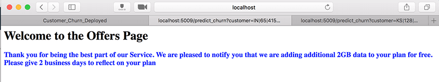
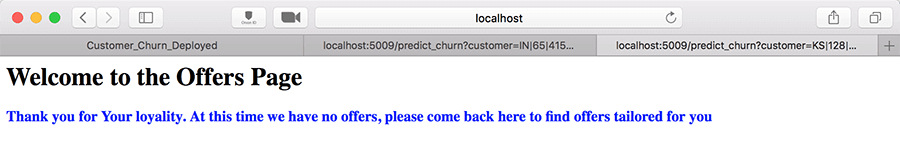
Given this is a simple demonstration of the capability, we will use any web browser with request parameters passed in the URL string. Imagine a customer is visiting an offers page on the customer portal and we are want to use our real-time customer churn prediction and present some tailored offers. Often such offers are tailored based on customer segments (customer segmentation is another topic of machine learning that is beyond the scope of this article).
The first URL below is where the model predicted a customer has a high propensity to churn, and the second URL is where the model predicted that the customer will remain loyal.
Real-time scoring of a Customer who has high propensity to churn
- https://localhost:5009/predict_churn?customer=IN|65|415|329-6603|no|no|0|129.1|137|21.95|228.5|83|19.42|208.8|111|9.4|12.7|6|3.43|4
Real-time scoring of a Customer who will remain loyal
- https://localhost:5009/predict_churn?customer=KS|128|415|382-4657|no|yes|25|265.1|110|45.07|197.4|99|16.78|244.7|91|11.01|10|3|2.7|1
This video demonstrates the deployment and real-time scoring using a local PySpark.
Conclusion
The real business value comes from leveraging both real-time and offline scoring to create machine learning models for targeted business outcomes. We hope you have learned how to deploy a model in Python using the Flask web service for real-time scoring. We recognize that this is not the only approach, and the same scenario can also be achieved using Java or Scala web service frameworks. If you have any questions about this set-up, please feel free to reach out to us at [email protected]
The technical content for this blog was curated using Qubole’s cloud-native big data platform and auto-scaling Spark clusters. Qubole offers you the choice of cloud, big data engines, tools, and technologies to activate your big data in the cloud. Sign up for a free Qubole account now to get started.