**Note: When using or referencing the content here, please be mindful of ESPNCricInfo terms of use.
At Qubole, we don’t just like cricket, we love it. Cricket is an ancient game that was invented in the 16th century. The Cricket World Cup is a tournament organized by the International Cricket Council (ICC) once every four years, the current edition of which started on May 30th, 2019, and is being held in England and Wales, UK.
In this article, using the cricket data available in the data-rich ESPNCricInfo portal, we will focus first on data wrangling to analyze the historical ODI player performances before diving into forecasting the performance of one of the top 10 cricketers for ICC Cricket World Cup 2019. Finally, we will predict the winner of the Cricket World Cup.
Data Acquisition and Wrangling
As a first step, the goal here is to analyze player performance using an interactive web form built using Qubole Notebook’s dynamic input forms capability with drop-downs that respond to a selection change by collecting/filtering the data associated with the selected player and refreshing the respective charts as demonstrated in the animated gif below.
On the ESPNCricInfo website, every player that has ever played international cricket is chronicled with a unique profile (player ID). for example: if you search for Virat Kohli, you will be linked to his profile page. The unique profile (player ID) of Virat Kohli can be inferred from the profile URL as 253802. The idea here is to start from the tournament squads page and acquire player metadata as well as historical batting/bowler data. For this purpose, we will use a simple and elegant Python package (BeautifulSoup) to parse and crawl the website pages.
After acquiring the cricket world cup 2019 squad list, The utility functions getCWCTeamData from a public GitHub repo file crawls through the squads’ page of each participating team (eg: the England Squad page) to acquire the player profiles. Following the acquisition of all player profiles, another utility function getPlayerData from the same GitHub repo Py file can be used to retrieve all of the historical batting/bowling records from stats.espncricinfo.com.
The below code block demonstrates the use of Python’s multiprocessing capabilities to independently and asynchronously acquire all of the player’s historical batting/bowling records. This fast-tracks the data acquisition and all of the historical data associated with every participating player in the ICC Cricket World Cup. On my Spark cluster master with 4 vCPUs and 30 gigabytes of memory, the average processing time was observed to be a little over three minutes on average, which is quite impressive.
import requests
import sys
import re
from lxml import html
from bs4 import BeautifulSoup
import pandas as pd
from multiprocessing import Pool
from pyspark.sql.types import *
from multiprocessing.pool import ThreadPool

url="https://raw.githubusercontent.com/Pradeep39/cricket_analytics/master/utilities/cricket_data_wrangling.py"
sc.addPyFile(url)
exec(requests.get(url).text)

batting_dfs=list()
bowling_dfs=list()

if __name__ == '__main__':
    pool=ThreadPool()
    #fetch worldcup squad list
    r = requests.get("http://www.espncricinfo.com/ci/content/squad/index.html?object=1144415")
    soup = BeautifulSoup(r.content, "html.parser")
    for ul in soup.findAll("ul", class_="squads_list"):
     for a_team in ul.findAll("a", href=True):
      team_squad_df = getCWCTeamData(a_team.text,\
                  "http://www.espncricinfo.com"+a_team['href'])

      for index, row in team_squad_df.iterrows():
        try:
            def getBatsmanCallback(resultDF):
                if not resultDF.empty:
                    batting_dfs.append(resultDF)
            pool.apply_async(getPlayerData, args = (row,"batting", ),\
                                callback = getBatsmanCallback)

            def getBowlerCallback(resultDF):
                if not resultDF.empty:
                    bowling_dfs.append(resultDF)
            pool.apply_async(getPlayerData, args = (row, "bowling", ),\
                                callback = getBowlerCallback)

        except Exception as ex:
          print("Exception in Main:"+str(ex))
          pass
    pool.close()
    pool.join()
Data Cleansing/ETL
All of the independently collected data associated with each player is not clean, so let’s use the distributed data processing power of Apache Spark by combining all of the data and projecting it to Apache Spark distributed memory for doing data cleansing in a distributed manner.
from pyspark.sql.types import *
from pyspark.sql.functions import *

batting_df = pd.DataFrame({})
bowling_df = pd.DataFrame({})

for df in batting_dfs:
    batting_df=batting_df.append(df)

for df in bowling_dfs:
    bowling_df=bowling_df.append(df)

batting_schema = StructType([StructField("Runs", StringType(), True),StructField("Mins", StringType(), True),StructField("BF", StringType(), True),StructField("4s", StringType(), True),StructField("6s", StringType(), True),StructField("SR", StringType(), True),StructField("Pos", StringType(), True),StructField("Dismissal", StringType(), True),StructField("Inns", StringType(), True),StructField("Opposition", StringType(), True),StructField("Ground", StringType(), True),StructField("Start Date", StringType(), True),StructField("Country", StringType(), True),StructField("PlayerID", StringType(), True),StructField("PlayerName", StringType(), True),StructField("RecordType", StringType(), True),StructField("PlayerImg", StringType(), True),StructField("PlayerMainRole", StringType(), True),StructField("Age", StringType(), True),StructField("Batting", StringType(), True),StructField("Bowling", StringType(), True),StructField("PlayerRole", StringType(), True)])

batting_spark_df=sqlContext.createDataFrame(batting_df,schema=batting_schema)

bowling_schema = StructType([ StructField("Overs", StringType(), True),StructField("Mdns", StringType(), True),StructField("Runs", StringType(), True),StructField("Wkts", StringType(), True),StructField("Econ", StringType(), True),StructField("Pos", StringType(), True),StructField("Inns", StringType(), True),StructField("Opposition", StringType(), True),StructField("Ground", StringType(), True),StructField("Start Date", StringType(), True),StructField("Country", StringType(), True),StructField("PlayerID", StringType(), True),StructField("PlayerName", StringType(), True),StructField("RecordType", StringType(), True),StructField("PlayerImg", StringType(), True),StructField("PlayerMainRole", StringType(), True),StructField("Age", StringType(), True),StructField("Batting", StringType(), True),StructField("Bowling", StringType(), True),StructField("PlayerRole", StringType(), True)])

bowling_spark_df=sqlContext.createDataFrame(bowling_df,schema=bowling_schema)

#distributed data cleansing operations to prepare data for analysis using matplotlib
clean_batting_spark_df = batting_spark_df\
     .filter("Runs!= 'DNB' AND Runs!='sub' AND Runs!='absent' AND Runs!='TDNB'")\
     .withColumn('Runs', regexp_replace('Runs', '[*]', ''))\
     .withColumn('Mins', regexp_replace('Mins', '[-]', '0'))

clean_bowling_spark_df = bowling_spark_df.filter(\
                          "Overs!= 'DNB' AND Overs!='TDNB'")
Interactive Analysis with Qubole Notebooks and Matplotlib
Batsman Performance Analysis
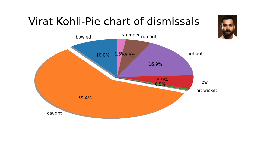
Now that we have a clean data set, any given batsman and bowler data can be filtered and collected back to the cluster master’s Python process for analyzing and plotting visualizations to provide better insights on player traits and trends. The below code block filters on Virat Kohli and plots a pie chart of his dismissals.
matplotlib.pyplot as plt
import seaborn as sns
from pylab import rcParams
from skimage import io

selectedPlayerProfile=253802

# Set figure size
rcParams['figure.figsize'] = 8,4

if selectedCountry==selectedPlayerCountry:
    batsman = clean_batting_spark_df\
             .filter(batting_spark_df.PlayerID == selectedPlayerProfile)\
             .toPandas()

    d = batsman['Dismissal']
    # Convert to data frame
    df = pd.DataFrame(d)
    df1=df['Dismissal'].groupby(df['Dismissal']).count()
    df2 = pd.DataFrame(df1)
    df2.columns=['Count']
    df3=df2.reset_index(inplace=False)

    image = io.imread(selectedPlayerImg)
    fig, ax = plt.subplots()
    explode = [0] * len(df3['Dismissal'])
    explode[1] = 0.1
    ax.pie(df3['Count'], explode= explode, labels=df3['Dismissal'],autopct='%1.1f%%',shadow=True, startangle=90)

    atitle = selectedPlayerName +  "-Pie chart of dismissals"
    plt.suptitle(atitle, fontsize=24)
    newax = fig.add_axes([0.8, 0.8, 0.2, 0.2], anchor='NE', zorder=-1)
    newax.imshow(image)
    newax.axis('off')
    z.showplot(plt)
    plt.gcf().clear()
Bowler Performance Analysis
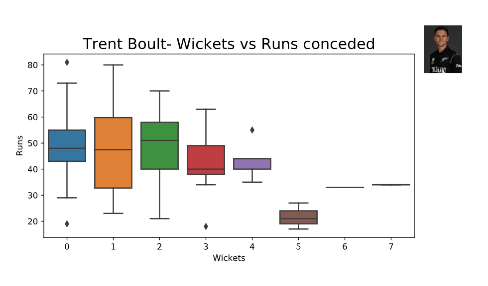
Let’s now focus on a bowler and analyze his historical performance. The below code block filters one of the top 10 bowlers — Trent Boult from New Zealand’s cricket team — and plots a box plot of the number of runs conceded per wickets taken.
import seaborn as sns
from pylab import rcParams
from skimage import io

selectedPlayerProfile=277912

bowler = clean_bowling_spark_df\
         .filter(clean_bowling_spark_df.PlayerID == selectedBowlerProfile)\
         .toPandas()

if not bowler.empty:
   bowler['Runs']=pd.to_numeric(bowler['Runs'])
   bowler['Wkts']=pd.to_numeric(bowler['Wkts'])
   # Set figure size
   rcParams['figure.figsize'] = 8,4
   image = io.imread(selectedBowlerImg)
   fig, ax  = plt.subplots()
   atitle = selectedBowlerName + "- Wickets vs Runs conceded"
   ax = sns.boxplot(x='Wkts', y='Runs', data=bowler)
   plt.title(atitle,fontsize=18)
   plt.xlabel('Wickets')
   newax = fig.add_axes([0.8, 0.8, 0.2, 0.2], anchor='NE', zorder=-1)
   newax.imshow(image)
   newax.axis('off')
   z.showplot(plt)
   plt.gcf().clear()
There are several other charts that can be built using the curated data. The interactiveness of selecting a player to see the respective charts and analysis was possible through Qubole Notebook’s dynamic forms capability.
Predictive Analytics: Predicting a Player Performance Using Time Series Analysis
Let’s dive into predicting/forecasting the future performance of a player. As a disclaimer, these predictions may be completely wrong and meant only to be referenced/used for educational purposes. Several variables impact player performance. Today we will explore a simple forecasting technique called “Time Series Analysis”. Time Series generally don’t require distributed scale processing as the series data is summarized and not of a big data class. While there are distributed time series libraries like spark-ts, they lack the breadth of what the Python Statsmodels package offers. So we shall stick with the Python Statsmodels package to complete this solution.
We will first focus on Time Series Analysis for one of the top batsmen in the world, Virat Kohli, to predict the runs he will score in the group stage of the tournament (round-robin stage). To cut to the chase, the time series model created produced the following predictions of runs scored by Virat Kohli in the group stages of the ICC Cricket World Cup:
########Virat Kohli world cup remaining group stage match runs predictions#######
#Bangladesh vs India on July 2nd: 67
#Srilanka vs India on July 6th: 67
#India vs Pakistan on July 9th: 67
#India vs Australia on July 14th: 66
##################################################################
There are several basic time series models like the Mean Constant Model which considers mean as the best prediction, the Linear Trend Model which fits a sloping line to predict the near future, and the Random Walk Model to predict the change from one period to the next. But we will focus our attention on one of the advanced time series models viz., ETS (Errors, Trends, and Seasonality) before jumping into time series analysis.
Most of the time series models work on the assumption that the time series is stationary. Intuitively, we can see that if a time series has a particular behavior over time, there is a very high probability that it will follow the same in the future. Also, the theories related to stationary series are more mature and easier to implement as compared to non-stationary series. The underlying principle behind these advanced models is to model or estimate the trend and seasonality in the series and remove those to get a stationary series. Statistical forecasting techniques can then be implemented on stationary series and the values can be forecasted and converted to the original scale by re-applying trend and seasonality constraints.
Before we move to the next step, we need to fill in the missing values. By missing values, I mean the calendar days where Virat Kohli has not played ODI cricket. The question we are trying to answer here is: how many runs would Virat have scored each calendar day since his career began if he played international ODI cricket every single day? There are several effective methods to fill missing values in a time series like mean/median imputation, rolling mean imputation, and imputation using different interpolation methods. We will go with imputation based on time-based interpolation. Below is the code to complete this step.
idx=pd.date_range(start=virat_df.index.min(), \
              end=virat_df.index.max(), freq='D')

virat_df = pd.DataFrame(data=virat_df,index=idx, columns=['runs'])

virat_df = virat_df.assign(RunsInterpolated=df.interpolate(method='time'))
Now that we have a clean, continuous time series, let’s look at a decomposition plot that will help us understand trends, seasonality, and residuals in the series. The below code completes this step and provides a chart that aids in analyzing the error, trends, and seasonality components of the series. To help avoid the noise, we will only look at the last few years of data in the series.
decomposition = seasonal_decompose(\
               virat_df.loc['2017-01-01':df.index.max()].RunsInterpolated)
decomposition.plot()
z.showplot(plt)
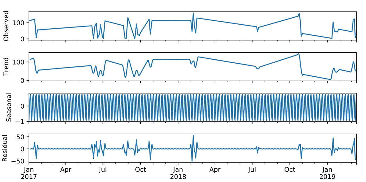
From the above decomposition plot, seasonality appears to be consistent over time with no apparent trend, and error/residual terms appear to be linearly varying over time. So when choosing one among the various advanced time series ETS models, based on the observations, we should choose ETS (A, N, A) due to the presence of Additive Error Terms, with no trend and additive seasonality. This class of ETS algorithms comes under the umbrella of Holt’s Winter Exponential Smoothing methods.
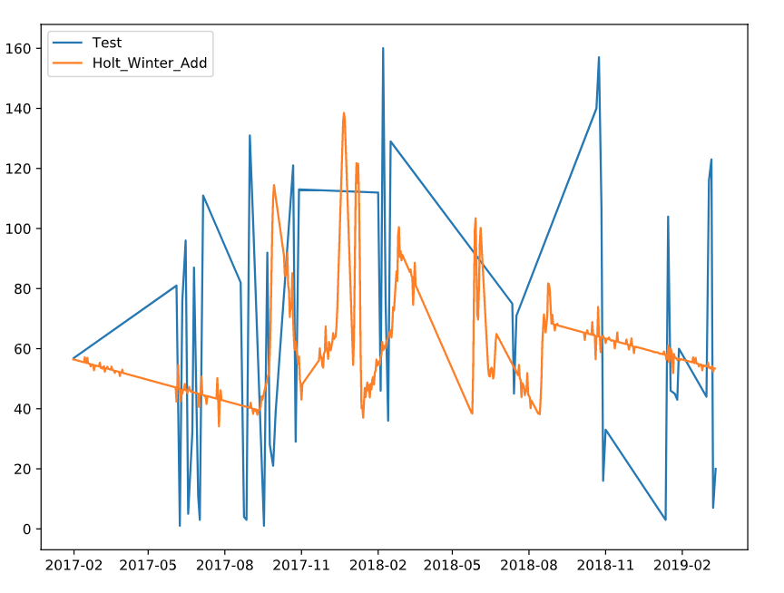
Note that to use Holt’s Winter Exponential Smoothing methods in Python, a specific version of statsmodels0.9.0rc1 (pip install statsmodels==0.9.0rc1) should be used. The below code block completes the step of splitting the series into train and test sets as well as model validation. The resulting graph helps us visually understand how close the model predictions are to the actual test values.
import matplotlib
from statsmodels.tsa.holtwinters import ExponentialSmoothing
rcParams['figure.figsize'] = 8,6
series=df.RunsInterpolated
series[series==0]=1
train_size=int(len(series)*0.8)
train_size
train=series[0:train_size]
test=series[train_size+1:]
y_hat = test.copy()
fit = ExponentialSmoothing( train ,seasonal_periods=730,\
                             trend=None, seasonal='add',).fit()
y_hat['Holt_Winter_Add']= fit.forecast(len(test))
plt.plot(test, label='Test')
plt.plot(y_hat['Holt_Winter_Add'], label='Holt_Winter_Add')
plt.legend(loc='best')
z.showplot(plt)
plt.gcf().clear()
The below block of code computes the RMSE (Root Mean Squared Error) for the fitted model. RMSE indicates the performance of the model in the test set.
from sklearn.metrics import mean_squared_error
from math import sqrt
rms_add = sqrt(mean_squared_error(test, y_hat.Holt_Winter_Add))
print('RMSE for Holts Winter Additive Model:%f'%rms_add)

#####Output#####
# RMSE for Holts Winter Additive Model:40.490023
Now let’s finally forecast out for 180 days beyond the last ODI game that Virat Kohli played and print the predictions for the runs that he will score in the group stage.
y_hat['Holt_Winter_Add']= fit.forecast(len(test)+180)
print('########Virat Kohli world cup match by match runs prediction 1 (Holts Winter Additive)#######')
print('########Virat Kohli world cup match by match runs predictions#######')
print('England vs India on June 30th: %d' \
                  %int(y_hat['Holt_Winter_Add'].loc['2019-06-30']))
print('Bangladesh vs India on July 2nd: %d' \
                  %int(y_hat['Holt_Winter_Add'].loc['2019-07-02']))
print('Srilanka vs India on July 6h: %d' \
                  %int(y_hat['Holt_Winter_Add'].loc['2019-07-06']))
print('###############################################################')

########Virat Kohli world cup match by match runs predictions#######
#Bangladesh vs India on July 2nd: 67
#Srilanka vs India on July 6th: 67
#India vs Pakistan on July 9th: 67
#India vs Australia on July 14th: 66
##################################################################

##################################################################
Predictive Analytics: Predicting the Winner of the World Cup
This GitHub repo file contains the recipe for predicting the winner of the world cup using Spark MLlib. To achieve this objective, the focus is to first gather all of the matches played since 1999 and build a binary response model based on those aggregated match metrics. We then score the model for the group stages to yield the below-projected points table. The model projects that England will lose to New Zealand to pave the way for Pakistan to enter the semi-finals.
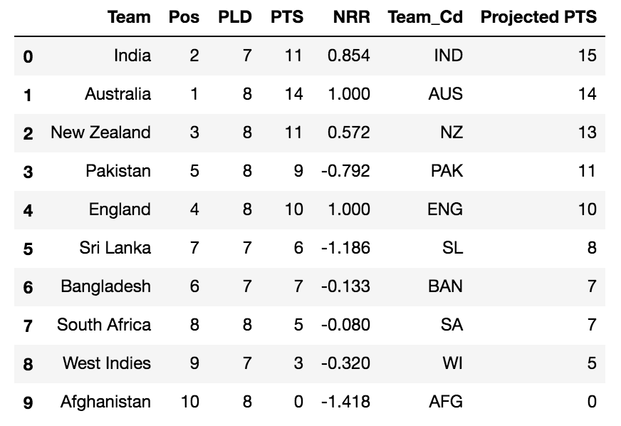
This then sets up an India-Pakistan semi-finals game at Old Trafford-Manchester on July 9th, and a New Zealand-Australia semi-finals game at Edgbaston-Birmingham on July 11th, where India and Australia will emerge as victors. Finally, the model predicts that Australia will win the world cup in the final to be held at Lord’s-London on July 14th between India and Australia. Below are the final results:
Probability of India Winning the final: 47%
Probability of Australia Winning the final: 53%
Win Prediction: Australia
Conclusion
This article demonstrated how to acquire data from a seemingly semi-structured source, transform/analyze player performance, and apply the time series predictive analytics technology to predict future player performance. Using these elements, we built a predictive model that forecasts who will win the world cup. For all of those cricket fans who have read this article thus far, enjoy the world cup, and may the best team win.