SQL Joins are a common and critical component of interactive SQL workloads. The Qubole Presto team has worked on two important JOIN optimizations to dramatically improve the performance of queries on Qubole Presto.
In this blog, we will talk about 2 join optimizations introduced in Qubole Presto:
- Join Reordering
- Dynamic Filtering
We also present improvement in the runtime of TPC-DS queries due to these join optimizations. Specifically, we show that:
- Join Reordering provides a maximum improvement of 6X.
- Dynamic Filtering provides 2.8X geomean improvement and 14X maximum improvement.
- Due to better resource utilization from these optimizations, Qubole Presto can now run 90 TPC-DS queries compared to 72 without these optimizations.
These optimizations have been added to QDS Presto version 0.180 and we are working with the open-source community to incorporate these optimizations back to open-source Presto code.
Performance Benchmark Setup
Our setup for running the TPC-DS benchmark was as follows:
TPC-DS Scale: 3000
Format: ORC (Non-Partitioned)
Scheme: HDFS
Cluster: 16 c3.4xlarge in AWS us-east region.
We ran the benchmark queries on QDS Presto 0.180. We have used TPC-DS queries published in this benchmark. To ensure that the benchmarks focus on the effect of the join optimizations:
- Default Presto configuration was used. For example, distributed joins are used (default) instead of broadcast joins.
- Data was stored in HDFS instead of S3
- No proprietary Qubole features like Qubole Rubix, autoscaling, or spot node support were used.
- Timings published are an average of 3 runs.
Join Reordering
Presto supports two types of joins – broadcast and distributed joins. In both cases,
- One of the tables is used to build a hash table. This table is called the build side and is typically notated on the right side.
- The other table is used to probe the hash table and find keys that match. This table is called the probe side and is typically notated on the left side.
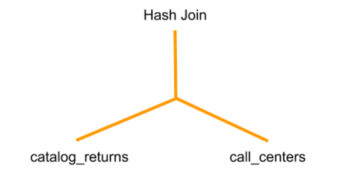
In the diagram above, call_centers is the build side and catalog_returns is the probe side.
For best performance, the smaller table should be on the build side and the larger table should be on the probe side. In the general case, the optimization is applicable for tables as well as subqueries or complex sub-trees as inputs to a join.
Until now, analysts using Presto were expected to ensure that the join order was correct [1][2]. While such an expectation was reasonable for simple queries, it is an impossible expectation for complex queries with many joins and subqueries. Analysts cannot guess the size of the resultset of a subquery!
The Join Reorder Module in Qubole Presto uses table and column statistics as well as a cost model to estimate the size of the inputs of a join and chooses the right order. In Qubole, users can generate statistics using the Automatic Statistics Collector.
Case study q91:
Let us take q91 as an example to illustrate how join reordering improves performance. The join tree of q91 without applying join reordering is shown in the figure below :
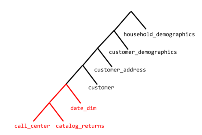
Every intermediate node in tree represents a join and every leaf node is a table. For every Join node left child represents the probe side and right side represents build side. Let us also look at the sizes on HDFS of each table below:
22.5 G /perf/data/tpcds/orc/scale_3000/catalog_returns
1.1 G /perf/data/tpcds/orc/scale_3000/customer
174.4 M /perf/data/tpcds/orc/scale_3000/customer_address
354.4 K /perf/data/tpcds/orc/scale_3000/date_dim
45.1 K /perf/data/tpcds/orc/scale_3000/customer_demographics
8.7 K /perf/data/tpcds/orc/scale_3000/call_center
896 /perf/data/tpcds/orc/scale_3000/household_demographics
In this case, the size on the disk is a good indicator that the catalog_returns is the biggest table. However, if we look at the plan above, we see that catalog_returns is on the build side of the join with table call_center. catalog_returns as the build side of a join is not a good choice and will have a detrimental effect on performance.
When we enabled join reordering, the planner chose the following join order:
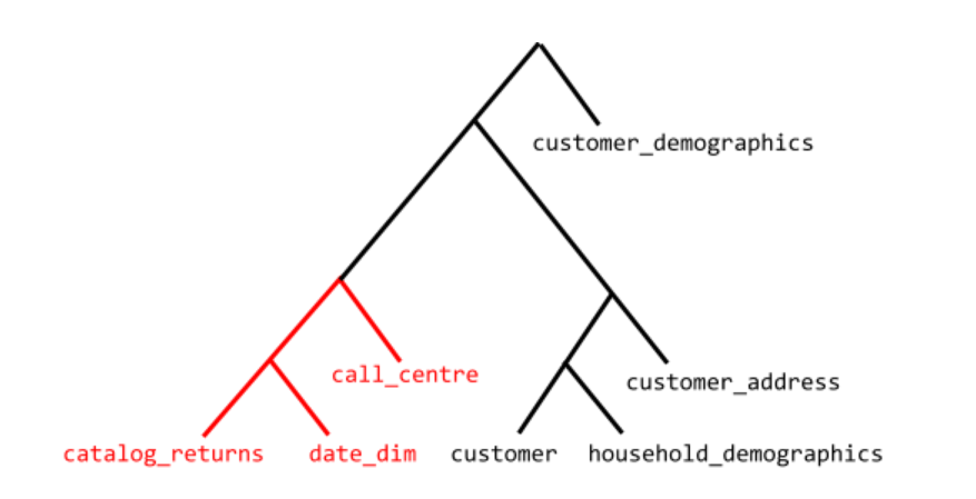
We can see above that catalog_returns is now on the probe side and call_centre is on the build side. The run time of the above query was reduced from 43 seconds to 7 seconds with join reorders enabled.
Improvements on TPC-DS queries:
- 17 queries that were failing earlier with Out of Memory errors without join reordering pass when join reordering is enabled. This shows that not only performance but join reordering can help to reduce the memory consumption of the queries.
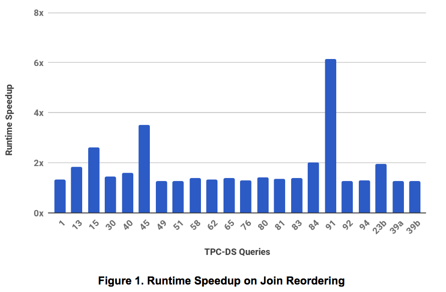
- Below figure shows 21 queries that saw more than 1.25x improvement on enabling join reordering:
Dynamic Filtering
Dynamic Filters remove rows from the probe (or large fact) table that will never match rows in the build table (or smaller dimension table). Consider the following query which captures a very common pattern of fact table joined with a dimension table.
SELECT * from fact_table A JOIN dimension_table B WHERE A.join_key = B.join_key;
Presto will push predicates for table dimension_table but scans all of table fact_table since there are no filters on fact_table.
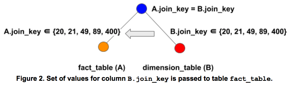
With Dynamic Filtering, Presto creates a filter on the B.join_key column, passes it to the scan operator of fact_table, and thus reduces the amount of data scanned in fact_table.
Dynamic Filters can be used to filter rows in the following scenarios:
- Partition pruning: In our example, if we assumed that A.date_key was a partition column, then dynamic filter A.date_key IN d” could have been used to prune partitions and save on I/O.
- Predicate Pushdown: When data is stored in columnar formats like ORC/Parquet, pushing predicates like A.date_key IN d” will reduce disk I/O.
- Filtering just after Table Scan: Filtering just after Table Scan can avoid sending more data to later operators and save on Network I/O and memory.
Experimental Evaluation
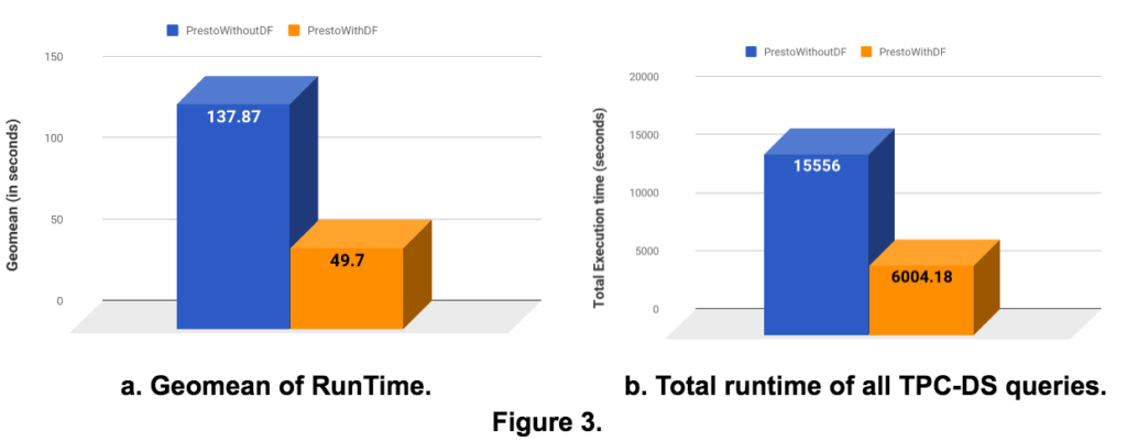
Dynamic Filtering (DF) improved the run time of many TPC-DS queries. We saw a 2.8x speedup in Geomean overall queries by applying Dynamic filtering (Fig. 3a). The total runtime obtained by summing up runtime for each individual query saw a speedup of 2.6x. The performance improvement varied by the query. To be more precise :
- The runtime of 13 queries improved by at least 5X.
- The runtime of 13 queries improved between 3X – 5X.
- The runtime of 22 queries improved between 1.5X – 3X.
- 14 queries that did not run before succeeded.
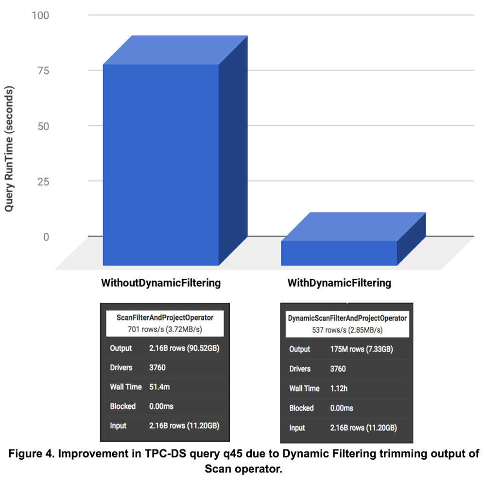
Case study q45:
Let us illustrate improvements in dynamic filtering through a deep dive into TPC-DS query q45. The figure below shows query runtime speedup of 8.3x with dynamic filtering. The figure also shows corresponding details of Scan operators (from presto UI) on fact table web_sales with and without Dynamic Filtering. Dynamic Filtering reduced the number of output rows of the Scan operator from 2.16B rows (90.52 GB) to 175M rows (7.33 GB), which resulted in much lesser data (12x) to be sent to further operators. The reduced number of rows resulted in an overall improvement of 8.3x in query runtime. Note that there is no partition pruning involved in this specific setup as the evaluation was conducted on non-partitioned tables.
Detailed evaluation on 104 TPC-DS queries is provided below:
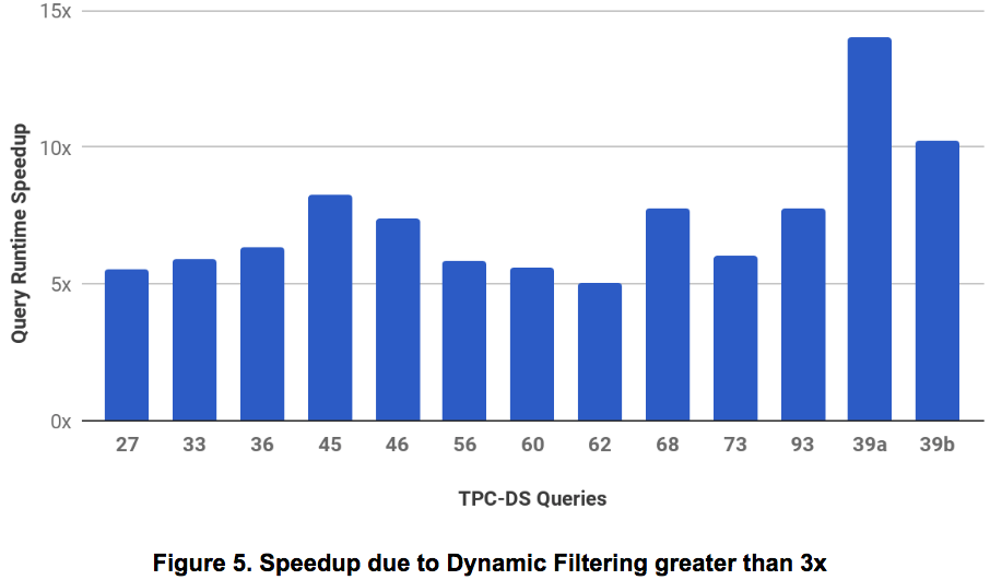
- Speedup greater than 5x: Figure 5 shows those 13 queries that showed more than 5x in runtime on applying Dynamic Filtering (DF).

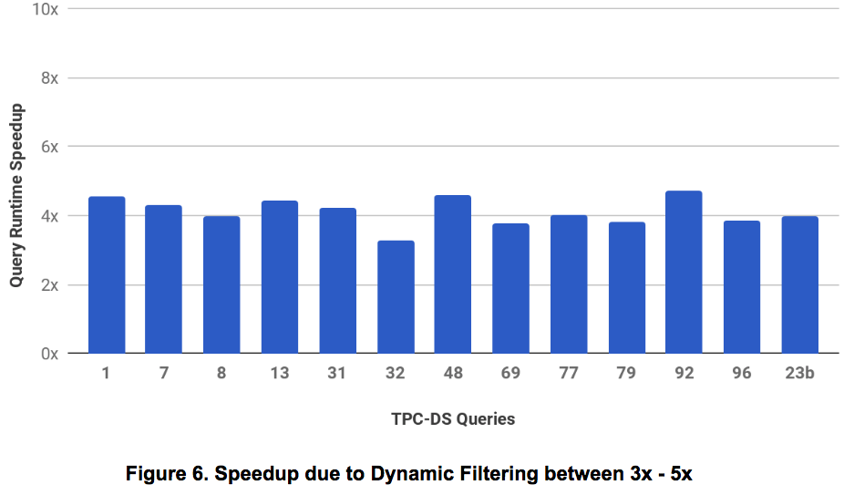
- Speedup between 3x – 5x: Figure 6 shows those 13 queries that showed more than 3x in runtime on applying Dynamic Filtering (DF).

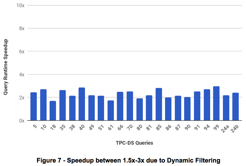
- Speedup between 1.5x – 3x: A total of 22 queries showed Speedup between 1.5x to 3x. Figure 7 captures those query speedup.

- Speedup less than 1.5x: Around 23 queries showed speedups lesser than 1.5 times and had insignificant effects due to dynamic filters.
- Queries that failed earlier and passing now: There were 14 queries that failed earlier without Dynamic Filtering and passes when Dynamic Filter is enabled. Out of 104 queries without Dynamic Filtering, we could run on only 72 queries and with Dynamic Filter, we could run on 86 queries. Queries were failing earlier due to OOM errors. Now with Dynamic filtering lesser data is sent to operators like Join causing lesser memory consumption and hence more queries passing than earlier.
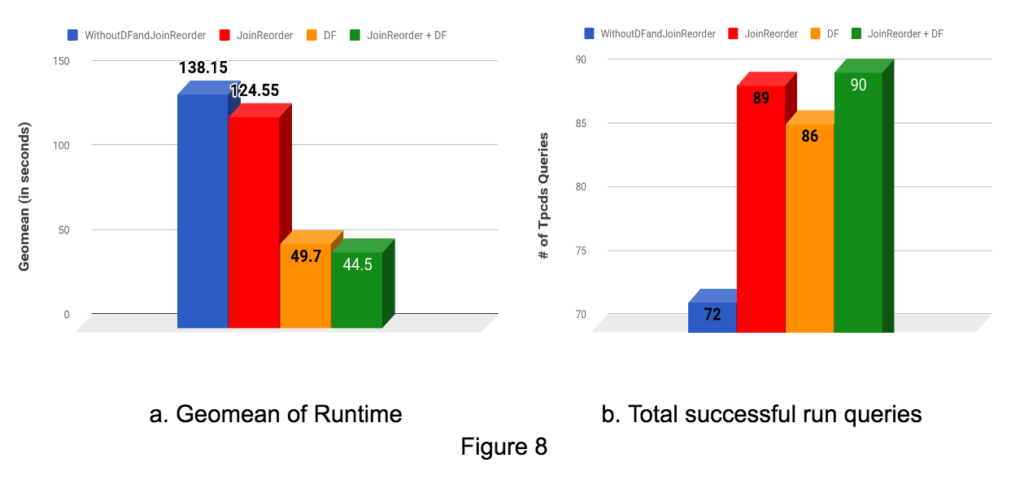
Cumulative Improvement with Join Reordering and Dynamic Filtering
The final result of applying both the optimization together can be seen in Figure 8 below. The first bar chart shows improvement in Geomean across all TPC-DS Queries ran. The second bar chart shows the number of queries that could run in different modes. We see 3.1x improvement with both join optimizations in Geomean and 18 more queries could run with the join optimizations.
Availability of Join Optimizations
Join reordering and Dynamic Filters have been added to Qubole Presto 0.180. To try it out sign up or please reach out to Qubole Support at [email protected].
Dynamic Filters has been discussed within the Presto community and there has been a very detailed design doc and some initial work on it. We have built on top of the work done by the community for dynamic filters. We hope to contribute Dynamic Filters back to the community and are working with Presto committers to add the feature to open source Presto. You can follow the progress here: https://github.com/prestodb/presto/pull/9453
Conclusion
This blog post explains the join optimizations we have added to Qubole Presto. Both the join optimizations provide dramatic performance (up to 14X) improvements on TPC-DS queries and datasets. Both these features are available on Qubole Presto now.
If you want to use a fast data engine for interactive analytics queries on cloud platforms like AWS & Microsoft Azure, check out Qubole’s Presto as a service.