Qubole just launched its Package Management feature, which is available on all of its Spark clusters. Package management makes it easy for data scientists to handle libraries, switch between Python and R versions, and reduce friction in the data science development cycle.
1. Why Do Data Scientists Use Libraries?
As a data scientist, I am always looking for more efficient ways to get my work done. Third-party libraries and packages allow me to progress, instead of getting stuck trying to solve problems that have already been solved. Whether it be Python, R, or Scala, each programming language has a rich set of libraries that help me get my work done. Qubole Spark clusters ship with the core libraries, but oftentimes I need additional libraries that may not be covered under the standard Java or Spark distributions. Below are a few commonly used libraries in Python and R:
| Task | Python Libraries | R Libraries |
| Visualization | Plotly, matplotlib | ggplot2 |
| Data prep | Pandas | dplyr, data.table |
| String parsing | BeautifulSoup | JSON |
| Machine Learning | Sci-kit Learn, TensorFlow | glmnet |
| Date/time handling | datetime | strftime |
Usually, I can take advantage of a library to accomplish every task. There are distributions that handle packages for both Python and R:
Python: https://anaconda.org/anaconda/repo
R: https://cran.r-project.org/
Only a few of these libraries such as H2O, XGBoost, Sparklyr, and SparkR have native integration with Spark, and most do not provide distributed capabilities.
Then what’s the point of using these libraries on distributed data?
I use these libraries in two ways:
- Jobs inside the driver
- Parallel jobs inside the executors
In the first case, I aggregate or sample the data into the driver for local in-memory processing such as visualization. In the second case, I often run non-distributed libraries inside Spark executors for parallel processing. For instance, running hyperparameter optimization by distributing local Scikit-learn jobs inside executors.
Handling packages and libraries are tedious, and I’ve spent a lot of my time worrying about how to handle libraries — which versions and packages to include in my environment. Moving code from one laptop to another or from one cluster to another often causes the code to break.
2. Qubole Package Management: Best in Class
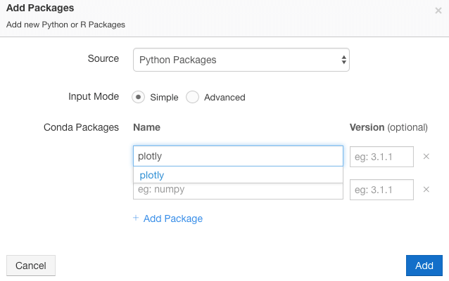
Before we launched Qubole Package Management, I had to manipulate the node bootstrap script to install libraries on my Spark clusters. For instance, if I wanted to install Plotly, a popular Python visualization library, I had to create a JIRA ticket and wait for the cloud administrator to add the following code into my node bootstrap script:
pip install plotly
And, having a custom script sitting in the cloud storage layer created many headaches for both myself and my cloud administrator. These include:
- Managing script versions
- Cluster startup due to dependencies being installed on the fly
- Cluster restart to add libraries
- A single script for multiple cluster configurations may cause unintended issues when changing the script
- Slowing down data science development — every change has to be approved and made by my cloud administrator
Qubole’s Package Management feature provides a graphical, secure, and intuitive interface to manage package dependencies. I can now create an environment that comes with the standard Conda distribution with around 40 different libraries.
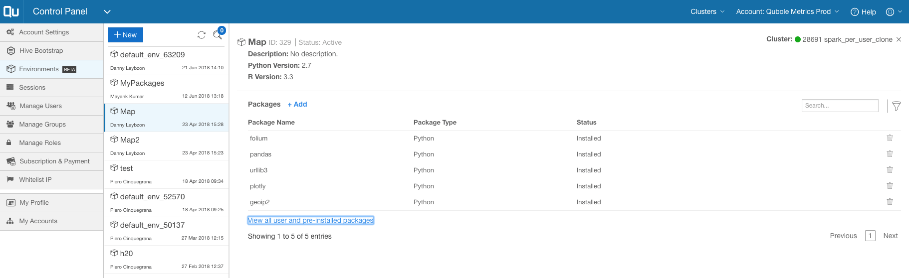
Each environment gets attached to a cluster, and package management lists the pre-installed R and Python libraries. I can add libraries on top of the standard distribution and easily manage the versions by adding and removing installed libraries. In most cases, this new feature eliminates the need to modify the node bootstrap.
3. Visualizing Financial Time Series Data
Let’s look at a real-world application of our package management feature. I demonstrate why the use of libraries arises in this financial services application.
I want to analyze a really interesting dataset from Deutsche Boerse. The dataset contains minute-level, stock-level data from 2017-06-24 to 2018-04-26 for stocks traded on the Eurex and Xetra trading systems. Here is the URL of the data for more information:
https://registry.opendata.aws/deutsche-boerse-pds/
3.1 Deutsche Boerse Dataset
The schema of the dataset is the following:
- ISIN: unique identifier for the stock
- Mnemonic: stock 3-letter ticker
- SecurityDesc: longer description of the security
- SecurityType: type of security (common stock, exchange-traded fund, exchange-traded commodity, exchange-traded note)
- Currency: currency in which the security is traded
- SecurityID: unique identifier for the stock similar to ASIN
- Date: day of the trade in the following format yyyy-mm-dd
- Time: The time when the trade happened in the following format HH:MM
- StartPrice: price at the beginning of the minute
- MaxPrice: maximum price within that minute
- MinPrice: minimum price within that minute
- EndPrice: price at the end of the minute
- TradedVolume: units of stock exchanged in that minute
- NumberOfTrades: number of trades within that minute (each trade could involve many units of stocks)
df = sqlContext.read.format("parquet").option("inferSchema","true"). load("path/to/file")
df.createOrReplaceTempView("deutsche")
Spark allows me to pass data frames through the sqlContext by issuing the following command createOrReplaceTempView. After calling this command, Qubole notebooks allow me to query the data directly with SQL. The ability to switch between Python and SQL allows me to pick the right language for every task. For instance, I prefer SQL to create simple queries involving joins, aggregations, and filtering, whereas Python is better for complex manipulations that require iteration and scripting.
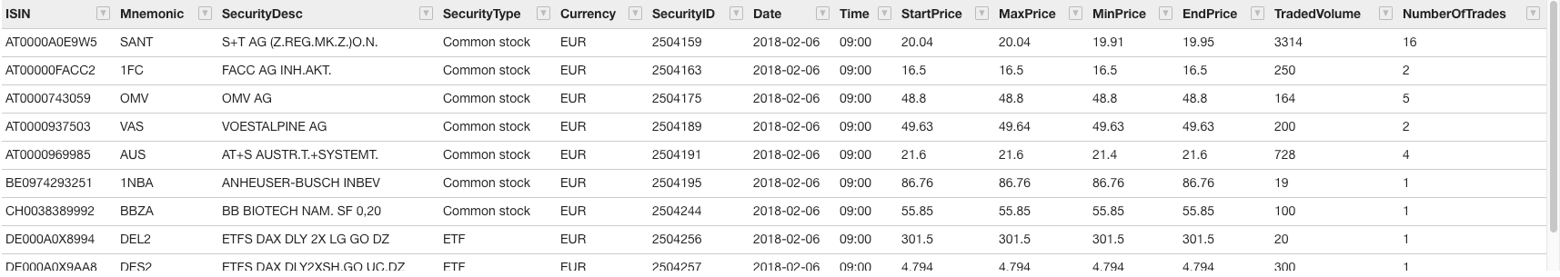
Here is how the data looks:
%sql
select * from deutsche limit 10
I am interested in understanding how much the price fluctuates within a minute. If there is a widespread (variation), it is an indication that there is a lot of trading activity at that minute.
%sql
select avg(MaxPrice-MinPrice) price_diff, Time from deutsche group by Time order by Time
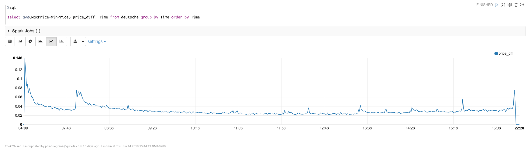
I then take the average price difference between MaxPrice and MinPrice and aggregate it by the column Time, i.e. by the minute. This gives me the following view: I see regular jumps throughout the day of the average difference at regular intervals, specifically every 30 minutes starting at 07:00 AM. One hypothesis for this pattern: algorithms programmed to do trades at regular intervals trigger other trades automatically, spurring a flurry of trading.
3.2 Using Package Management with Financial Data
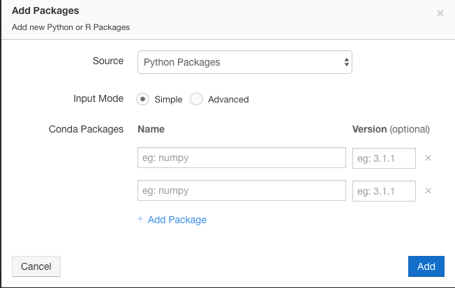
Qubole notebooks provide out-of-the-box capabilities to plot Spark data frames registered in the sqlContext. In this case, I want to explore the dataset further by creating a more complex visualization that requires Plotly, NumPy, and Sklearn. In order to do this, I am going to add the package plotly to the environment attached to this cluster and the package will become immediately available in the notebook.
Next, I will aggregate the data at the stock level, so it fits in memory, and convert the Spark data frame into Pandas, which collects the data into the driver.
import numpy as np
import plotly
import plotly.graph_objs as go
from sklearn import linear_model
pandas_df = sqlContext.sql("select * from (select Mnemonic, sum(TradedVolume) volume, avg((MaxPrice - MinPrice) / MinPrice) volatility from deutsche group by Mnemonic) where volume<>0.0")
pandas_loc = pandas_df.toPandas()
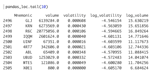
pandas_loc['log_volatility'] = np.log(pandas_loc.volatility+0.01)
pandas_loc['log_volume'] = np.log(pandas_loc.volume+0.01)Taking the log of the two series allows me to better visualize the relationship, given that the distributions are very skewed. Here is how the data looks:
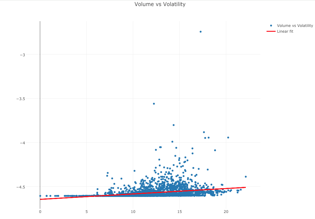
After a few steps, I obtain a beautiful scatterplot with a linear regression fit that helps me understand the relationship between trading volume and implied volatility as measured by intra-minute percent deviation of price.
x = pandas_loc.log_volume.reshape(2506,1)
y = pandas_loc.log_volatility.reshape(2506,1)

# Create linear regression object
regr = linear_model.LinearRegression()

# Train the model using the training sets
regr.fit(x, y)
pandas_loc['prediction'] = regr.predict(x)
trace1 = go.Scatter(
    x = pandas_loc['log_volume'],
    y = pandas_loc['log_volatility'],
    mode = 'markers'
)
trace2 = go.Scatter(
    x =  pandas_loc['log_volume'],
    y = pandas_loc['prediction'],
    mode = 'lines',
    line=dict(color='red', width=3)
)
layout = dict(
        title = 'Volume vs Volatility',
        showlegend = True,
        height = 800,
        width = 1050
    )
data1 = [trace1, trace2]
fig1 = dict( data=data1, layout=layout )
plot(fig1,  show_link=False)
Conclusion
Managing environments is an essential part of any data science project. Qubole’s Package Management feature allows me to easily manage and update libraries, switch between language versions, and reduce frictions in the data science development cycle. Qubole notebooks — combined with Package Management — make it easy to query, manipulate, visualize, and summarize data at scale.