In this post, we describe the design and implementation of a memory cost model in Qubole Presto, which when provided with a query and relevant table statistics, estimates the maximum memory requirements for that query.
A memory cost model can be used to solve problems such as:
- To evaluate and choose memory-efficient plans in Cost-Based Optimizers.
- Supervised Admission Control
- Cost aware Task Schedulers (to maximize memory utilization)
- Progress monitoring
For instance, Join Order optimization available in Qubole Presto uses the cost model described in this blog to select the best join order for a query.
The accuracy of the cost model is important as well. A bad estimate can lead to suboptimal or even confusing decisions. Prior literature provides an overview of problems and solutions to errors in statistics and query cost models. To mitigate such errors, we ran a sequence of validation experiments to improve estimates of our cost model using benchmarks and synthetic data and introduced a few heuristics such as guessing the join type to be the foreign key type if a number of rows are the same as the number of distinct values. We found that the correctness of our cost model is within a factor of 2 of actual usage in the worst case of memory for non-skewed data.
Need for a Resource Cost Model
In distributed systems, accurate resource estimation is key to making proactive scheduling and resource provisioning decisions in the system, thereby improving its overall efficiency and performance. Predominantly, system resource consumption is measured in terms of memory, CPU, network, and I/O bandwidth during execution. Due to Presto’s pipelined, mostly in-memory and non-containerized architecture, query completion relies heavily on the availability of required resources. Scheduling and resource provisioning decisions based on estimates of a cost model can greatly improve the chances that a query will have sufficient resources to execute.
In Presto, Join and Aggregate operators are the most resource expensive operators with memory being the most contented resource. These operators use in-memory hash-based data structures to speed up execution and hence require relatively much more memory to execute. To solve this problem, we decided to build a cost model based on peak memory usage. However, the framework we discuss below is generic enough to be extended to other resources like CPU and I/O in the future.
Applications in Qubole Presto
Qubole Presto uses the memory cost model for the following features:
- Cost-Based Optimizer: In Presto, insufficient memory resources for even one task can lead to query failure. Therefore, a memory-efficient plan is extremely critical for query success. We have implemented Join Ordering on top of this work to select the most memory-efficient plan in Qubole Presto.
- Admission Control: Presto uses a pipelined architecture where the complete query plan is instantiated and queries obtain resources from a shared pool. Due to this, capacity planning and admission control become imperative for predictable performance. The problem is exacerbated in highly concurrent environments where queries fired by one user can end up impacting queries from other users. To mitigate this and provide performance isolation, we have implemented admission control in one of our services using the cost model described in this blog. We use the upper bound of memory estimates from the cost model to reserve memory requirements for each query and schedule only those queries that have their resources available, which in turn, ensures predictable performance.
In our future work, we hope to use this cost model as a foundation for other features such as:
- Autoscaling cluster size on the basis of resource requirements. Recommending cloud instance types (based on memory) to be used for a given workload (batch of queries).
- Ensuring predictable performance by minimizing memory contention among queries by smarter scheduling of tasks. Presto currently supports query queues and resource groups. While they do help in ensuring system stability and resource isolation, these mechanisms are reactive in nature and will fail a query if it goes beyond its resource limits instead of using proactive admission control and intelligent scheduling to ensure performance isolation.
- Given the workload, auto-tuning parameters such as reserved-memory and query-peak-memory-per-node ensure successful completion.
Approach
For each query submitted, Presto creates a Logical Plan which is basically a DAG of tasks that can be executed in parallel, pipelining the intermediate results. Presto then uses the logical plan and table metadata to generate a Distributed Plan (with task → node assignments) consisting of Plan Fragments. A Plan Fragment consists of a set of operators running in parallel on the same node in a pipeline.
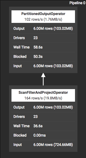
An operator pipeline snapshot from Presto UI (Snapshot 1)
Snapshot 1 shows a plan fragment where ScanFilterAndProjectOperator is responsible for scanning data from underlying data sources (e.g., s3), filtering it, and then projecting the required columns, one page at a time, to the consuming operator. It then passes this data to PartitionedOutputOperator, which is responsible for partitioning this data and distributing it to consumers of this pipeline.
Illustration with a simplified example:
Let us consider the DAG below-representing operator dependencies.
- Each node here represents an operator.
- An edge between node i and j (Eij) represents operator i consuming output produced by operator j.
- Accumulating Operators, as the name suggests, are the ones that accumulate data in underlying data structures, process it, and then return results only after processing all of the input data (e.g., sort, join). These are marked in red (operator B) and have higher costs (10).
- Pipelining Operators operate on one page at a time and are marked in green (operators A, D, E, F, and G). Their memory cost is assumed to be 1 unit.
- Partially Accumulating Operators are operators which accumulate data from one of the input sides and then stream data from another side (operator C). HashJoinOperator for example accumulates data from the left child in hashes and arrays and then streams the output from the right child to join one page at a time.
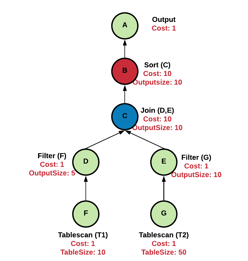
Figure 1: Operator Dependency DAG
Consider a query of the form:
Select T1.c3, T2.c3 from T1 join T2 on T1.pk = T2.pk where T1.a = “XXX” and T2.a=”XXX” order by T1.c2
Figure 1 shows the DAG corresponding to this:
- Node B and E cannot be active simultaneously as join node C first accumulates the output of node E in hash tables and only after that starts producing results.
- There is an indirect dependency between D and E. C will start consuming data from the left side (D) only after it has consumed all from the right side (E).
- B, C, D, and F can be active simultaneously, where B consumes the output of C, C of D, and so on.
- In this example, the scenario leading to maximum memory consumption will be when nodes B, C, D, and F are active simultaneously which is (10+10+1+1 = 22 units).
Algorithm/Implementation
At a high level, our implementation in Presto consists of the following steps:
- Establish one-to-one mapping between nodes in the logical and distributed plans.
- Calculate input and output statistics of each operator recursively.
- Calculate the memory requirements of each operator on the basis of these statistics and data structures used by the operator’s execution logic.
- Calculate memory requirements over a maximal set of operators which can execute concurrently.
The algorithm, starting from leaf nodes, considers a sub-tree of the current root node and calculates maximal memory requirements of any combination of nodes running in the sub-tree.
For a given sub-tree, we keep track of 2 values:
- The maximum memory requirement of the sub-tree (maxMem).
- Maximal memory requirement when root node is active (maxAggregateMemWhenRootActive).
Performing a post-order/depth first traversal, we calculate the values for node under consideration as follows:
At each step, we update:
- maxAggregateMemWhenRootActive :
maxAggregateMemWhenRootActive = self.memReq
For each child ∈ this.children
If child.accumulating:
maxAggregateMemWhenRootActive += child.memReq
else:
maxAggregateMemWhenRootActive += child.maxAggregateMemWhenRootActive - maxMem = Max(maxAggregateMemWhenRootActive, ∑child.maxAggregateMemWhenRootActive)
This algorithm updates maxAggregateMemWhenRootActive of the root node (of the sub-tree under consideration) to be the summation of one value corresponding to each child and the operating cost of the node. If the child is an accumulating node, we consider only the child’s operating cost since descendants have completed processing. If the child is a page processing node, then we consider its maxAggregateMemWhenRootActive which in effect makes sure that all active nodes in the child’s descendants are considered.
Results
We evaluated the correctness of our memory cost model through experiments comprising of running queries from the TPC-DS benchmark. The experiment setup is as follows:
- Queries are from a subset of the TPC-DS benchmark (scale 10,000)
- Cluster size: 1 master and 5 slaves, each of type r3.4xlarge in AWS
- Numbers reported from presto are peak memory across clusters, whereas estimator output is per node. Hence, for comparison, we have used Peak_Mem/Slave_Count
- For queries that consumed less than 100MB, estimates deviated from actual results by a margin of less than 50 MB (12 queries)
- We have assumed standard costs for table scan operators by using back-of-the-envelope calculations on the basis of data format and have not included it in result comparisons.
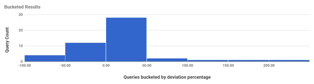
Figure 2: Queries by deviation percentage
Figure 2 shows a histogram of a number of queries bucketed by the percentage by which our estimation was off. For most queries, our estimation was within 50% variation from actual memory requirements, mostly erring on the over-approximation side. We over-approximate by design as this allows us to handle worst-case scenarios.
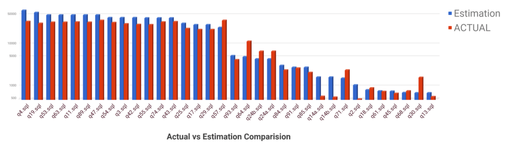
Figure 3: Actual vs Estimated Memory (MBs) Comparison
Figure 3 shows the actual vs estimated memory used (in Mbs) for TPC DS queries on a logarithmic scale. Consider q45.sql for example, the Blue bar shows the estimated value, which was 775Mb, and the Red bar shows the actual memory usage, which was 664Mb. As evident from the graph, for certain queries ex: q30.sql (second from right) the difference between estimated and actual memory used is huge – these represent potential areas of improvement and we are working on them.
Conclusion
Query cost models are the foundation of many important features in data processing. The accuracy of a cost model is also very important. A bad estimate can lead to suboptimal or even confusing decisions. In this post, we described the design and implementation of a memory-based cost model for Presto and experimentally demonstrated that it has reasonable accuracy for the features we have built with it. Currently, we assume the worst-case scenario for each node and are over-approximate – however, this is unlikely to occur in practice. We continue to fine-tune and further improve our cost model using real usage data.
If you find such problems interesting, we are always looking for great engineers. Check out Qubole’s career page.