This notebook will walk you through the process of building and using a time-series analysis model to forecast future sales from historical sales data. In particular, it will cover the use of PySpark within Qubole’s environment to explore your data, transform the data into meaningful features, build a Random Forest Regression model, and utilize the model to predict your next month’s sales numbers. For this notebook, we are providing a complete solution to Kaggle’s Predict Future Sales challenge.
Setting Up the Environment
Our first task is to set up our environment inside Qubole. We create a notebook in three easy steps:
- Click New.
- Provide a name.
- Select the appropriate language and version number. For this particular example, we choose PySpark (v2.1.1).
Now that we have access to a development environment, we can start building the predictive model. The first step is to create a collection of historic sales data. We have uploaded the data from the Kaggle competition to an S3 bucket that can be read into the Qubole notebook.
The process to convert this historic data set into a predictive model (shown in Figure 1 below) will include the following steps:
- Data ingestion and visualization
- Data cleanup and table joining to create single feature vectors
- Data preparation including feature discovery
- Model creation, training, and validation
- Prediction of future sales
The historic data is stored within an AWS S3 bucket and is ingested and visualized to allow the user to understand the scope and breadth of the available data. The data must be cleaned and combined into a collection of single feature vectors for each inventory item at the level of interest for prediction (for example, the per store item inventory being sold). The data is then prepped for use in training the model.
The key part of this preparation is the selection and discovery of key temporally variant features that may be useful in predicting sales numbers (e.g. the average sales of each item over the past three months). Last month’s numbers are then extracted for future use in predicting next month’s sales numbers, and numbers from the four months prior to that are set aside for model validation. The remaining historic data is used to train the Random Forest Regression model. The accuracy of the model is then measured and the model is used to predict the company’s sales numbers for the next month.
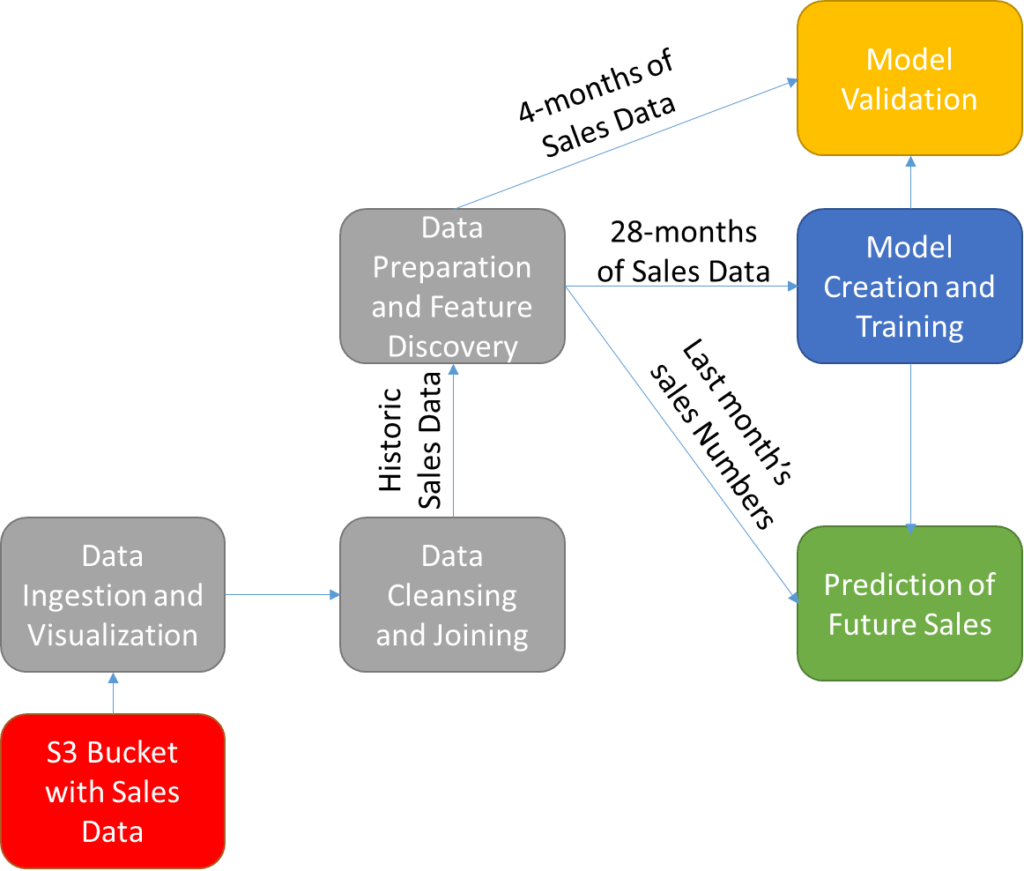
Figure 1: An overview of the process for training and utilizing a sales prediction model trained on time-variant historical sales numbers.
Step 1: Ingestion of Historic Sales Data
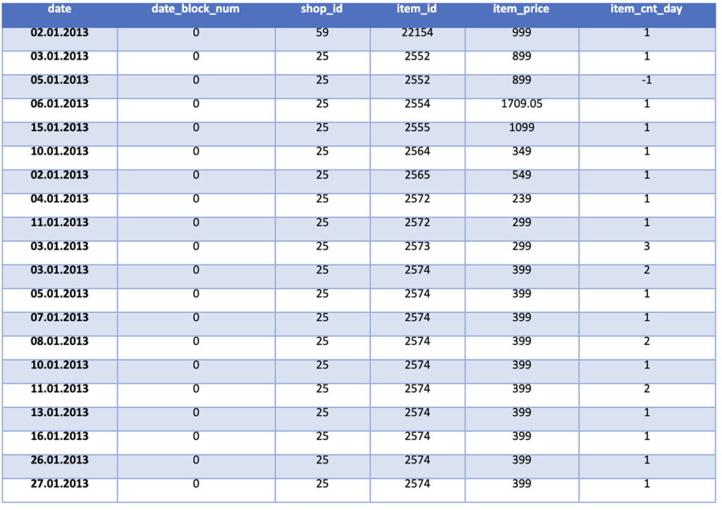
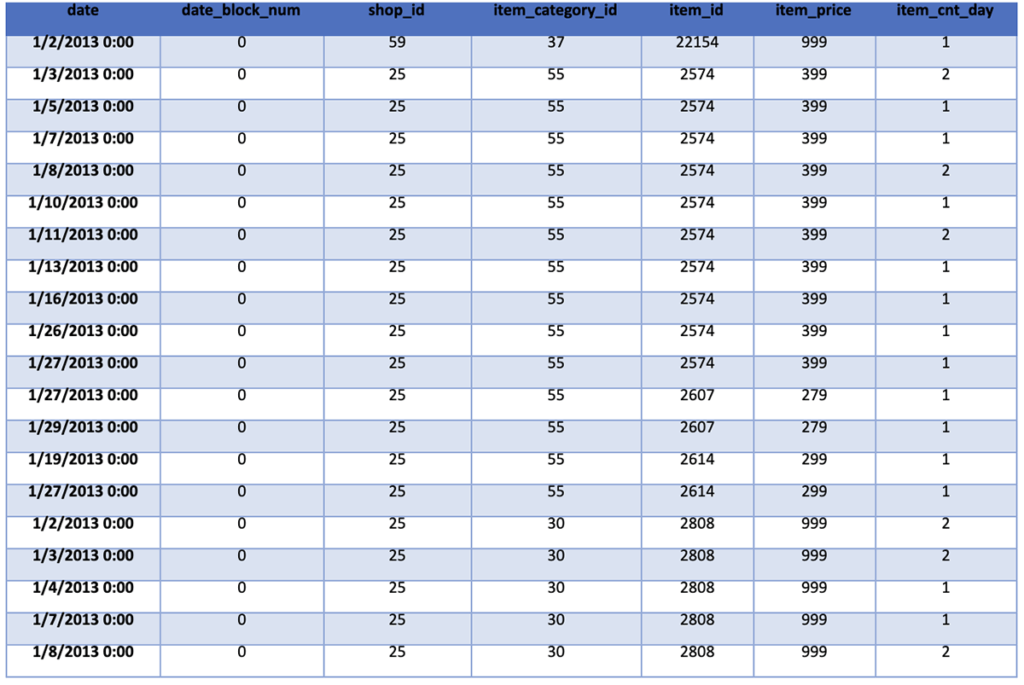
Before we can start, we first need to access and ingest the data from its location in an S3 datastore and put it into a PySpark DataFrame (for more information, see this programming guide and select Python tabs). This data includes historic sales, inventory (items) data, categories of items, and shop information. We also visualize the top 20 rows of the imported historic sales data to see what type of information we have available to us.
%pyspark

sales_train_file = "s3://salestestdata2/sales_train_v2.csv"
cat_file = "s3://salestestdata2/item_categories.csv"
items_file = "s3://salestestdata2/items.csv"
shops_file = "s3://salestestdata2/shops.csv"
test_file = "s3://salestestdata2/test.csv"

sales_train = spark.read.csv(sales_train_file, header=True, inferSchema=True)
categories = spark.read.csv(cat_file, header = True, inferSchema = True)
items = spark.read.csv(items_file, header = True, inferSchema = True)
shops = spark.read.csv(shops_file, header = True, inferSchema = True)
sales_test = spark.read.csv(test_file, header = True, inferSchema = True)
sales_train.show()
Step 2: Data Cleanup and Table Joining to Create Single Feature Vectors
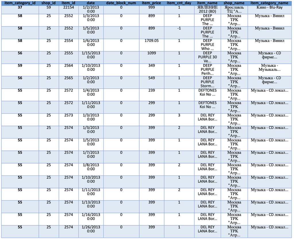
A key finding from looking at the historical data is that the format of the data will require some manipulation (the data field) and casting to best support the training process. Therefore, we create a short function to cast the data frame based on the column ID. Once the data is recast and formatted, we then want to combine the information from the sales, category, item, and shop files into a single data frame.
We accomplish this goal through joining the data frames on the appropriate unique IDs (item_id, shop_id, and item_category_id). We then count the number of entries and print the resulting combined data frame.
%pyspark
from pyspark.sql import types, functions as F
from pyspark.sql.functions import unix_timestamp
def cast_types(df):
dtypes = df.dtypes
if "ID" in df.columns:
df = df.withColumn("ID", df["ID"].cast(types.IntegerType()))
if "date" in df.columns:
#df = df.withColumn("date",df['date'].cast(types.DateType()))
df = df.withColumn("date", F.from_unixtime(unix_timestamp('date', 'dd.MM.yyyy')))
if "date_block_num" in df.columns:
df = df.withColumn("date_block_num", df["date_block_num"].cast(types.ByteType()))
if "shop_id" in df.columns:
df = df.withColumn("shop_id", df["shop_id"].cast(types.ByteType()))
if "item_id" in df.columns:
df = df.withColumn("item_id", df["item_id"].cast(types.ShortType()))
if "item_price" in df.columns:
df = df.withColumn("item_price", df["item_price"].cast(types.FloatType()))
if "item_cnt_day" in df.columns:
df = df.withColumn("item_cnt_day", df["item_cnt_day"].cast(types.FloatType()))
return df
%pyspark
sales_train = cast_types(sales_train)
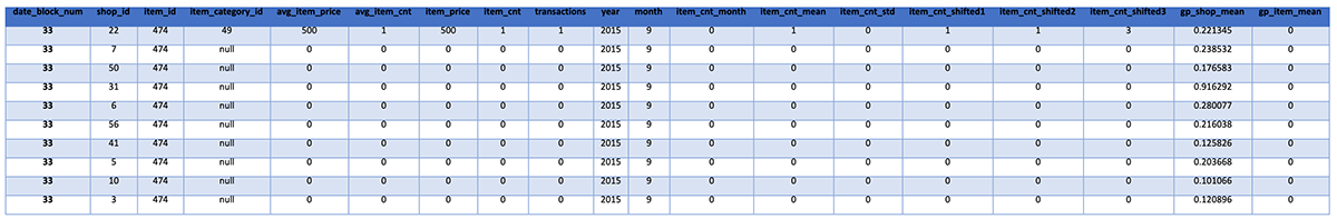
train = sales_train.join(items, on='item_id').join(shops, on='shop_id').join(categories, on='item_category_id')
print(train.count())
train.show()
Item Count: 2,925,510
Our next step is to remove items that are no longer being sold and shops that are no longer open. In our case, we know this information because they are not listed in the test file. However, in reality, the company developing the model would be aware of this information.
We count and print the number of rows in our initial data set for comparison once the old items and shops are removed. We then filter based on the list of unique items and shop IDs in the test data frame. The resulting training set is a significant subsection of the initial as many items and shops are no longer relevant. We then print the updated data frame for reference.
%pyspark
print('Initial Training Set Size: %s' % train.count())
test_shop_ids = sales_test.select('shop_id').distinct()
test_item_ids = sales_test.select('item_id').distinct()
train_filtered = train.join(test_shop_ids, "shop_id")
train_filtered = train_filtered.join(test_item_ids, "item_id")
print('Filtered Training Set Size: %s' % train_filtered.count())
train_filtered.show()
Initial Training Set Size: 2,925,510
Filtered Training Set Size: 1,221,909
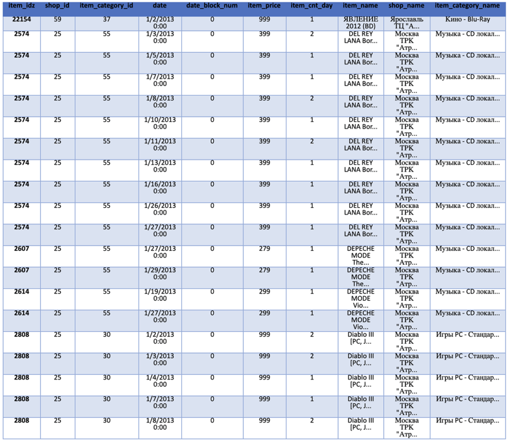
Our next step is to remove the text-based fields from the data frame. While they could provide additional information and improve our overall accuracy, we will ignore them for this notebook. (If you are interested in using this information, each of the fields actually contains multiple pieces of information. For example, the shop name includes the location of the shop as the first part of the name.) We then show the updated data frame with the limited attributes.
%pyspark
train_monthly = train_filtered[['date', 'date_block_num', 'shop_id', 'item_category_id', 'item_id', 'item_price', 'item_cnt_day']]
train_monthly.show()
Step 3: Data Preparation Including Feature Discovery
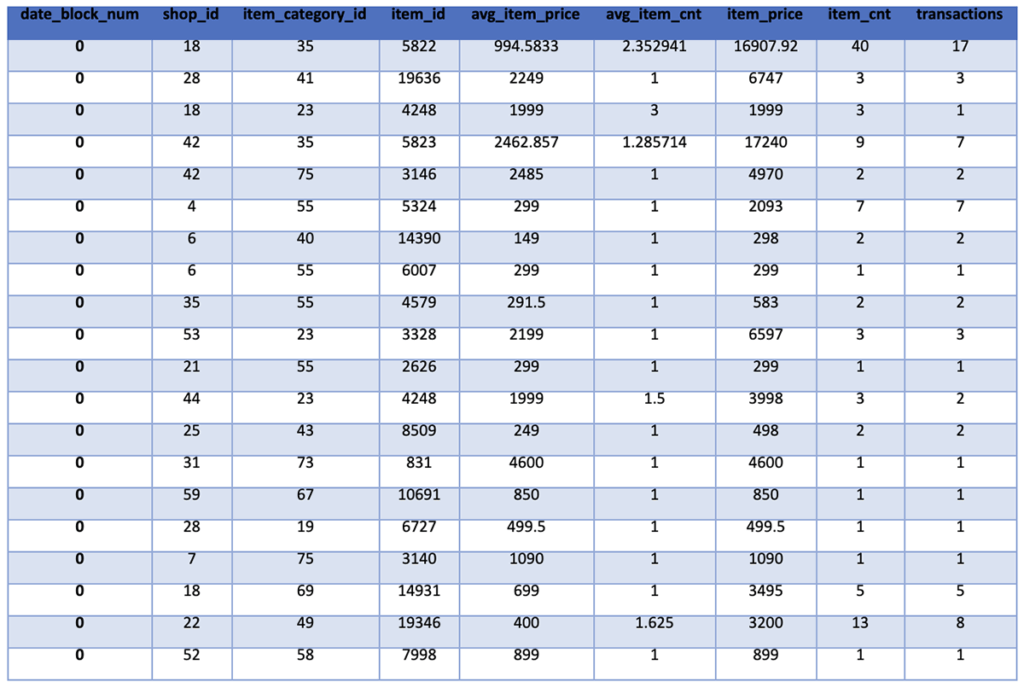
Now that we have a finalized version of the input data, our next goal is to prepare the data for use in training our model. Our first step will be to calculate the average values for each item’s price and sales counts, the total cost and an item count of each item transaction, and the total number of transactions including each unique item.
To accomplish this goal, we will sort the transactions by date and then group them by the month of the transaction, the shop, the item category, and the item. We then aggregate the data while calculating the desired means, sums, and counts. The resulting data frame is then shown for review.
%pyspark
group = train_monthly.sort('date').groupby("date_block_num", "shop_id", "item_category_id", "item_id")
train_monthly = group.agg(F.mean('item_price').alias('avg_item_price'), F.mean('item_cnt_day').alias('avg_item_cnt'), F.sum('item_price').alias('item_price'), F.sum('item_cnt_day').alias('item_cnt'), F.count('item_cnt_day').alias('transactions'))
train_monthly.show()
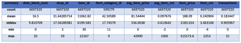
In the future, there are likely to be items sold at shops that have not previously been sold in that shop. To ensure our training data includes all possible item-shop combinations, we create a new data frame that includes all unique item-shop combinations and join this with our training data. For simplicity, we simply set all values for the new item-shop combinations to 0. However, it would be more accurate to set these to the appropriate average values based on the item averages we just calculated. We then show the statistics for the data frame for review.
%pyspark
from pyspark.sql.types import *
shop_ids = train_monthly.select('shop_id').distinct().collect()
item_ids = train_monthly.select('item_id').distinct().collect()
%pyspark
shop_item_pairs = []
for i in range(34):
    for shop in shop_ids:
        for item in item_ids:
            shop_item_pairs.append([int(i), int(shop.__getitem__('shop_id')), int(item.__getitem__('item_id'))])
shop_item_pairs = spark.createDataFrame(shop_item_pairs, ['date_block_num','shop_id', 'item_id'])
%pyspark
train_monthly = shop_item_pairs.join(train_monthly, on=['date_block_num','shop_id','item_id'], how='left')
train_monthly = train_monthly.fillna(0)
%pyspark
train_monthly.describe().show()
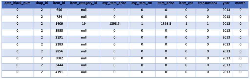
Given the knowledge that the data is split by month and our goal is to predict the next month’s sales number, we next utilize the data_block_num field to create Year and Month fields for each row. We then display the updated data frame for review.
%pyspark
year = F.udf(lambda x: ((x//12) + 2013), IntegerType())
month = F.udf(lambda x: (x % 12), IntegerType())
train_monthly = train_monthly.withColumn("year", year(train_monthly.date_block_num))
train_monthly = train_monthly.withColumn("month", month(train_monthly.date_block_num))
train_monthly.show(10)
We then finish our data preparation and feature creation step by removing outliers, adding features for the average and standard deviation of item counts for each Shop-Item Category-Item set and adding features for the past three months of item sales for each Shop-Item Category-Item set. For outliers, we determined that anything with a negative item count or an item count above 20 and anything with a price above 400,000 is an outlier.
%pyspark
from pyspark.sql import Window
train_monthly = train_monthly.filter('item_cnt >= 0 and item_cnt <= 20 and item_price < 400000')
train_monthly = train_monthly.withColumn("item_cnt_month", F.lag("item_cnt",1).over(Window.partitionBy("shop_id", "item_id").orderBy("date_block_num")))
%pyspark
train_monthly = train_monthly.withColumn('item_cnt_mean', F.avg('item_cnt').over(Window.partitionBy("shop_id", "item_category_id", "item_id").orderBy("date_block_num").rangeBetween(-2,0)))
train_monthly = train_monthly.withColumn('item_cnt_std', F.stddev('item_cnt').over(Window.partitionBy("shop_id", "item_category_id", "item_id").orderBy("date_block_num").rangeBetween(-2,0)))
%pyspark
train_monthly = train_monthly.withColumn("item_cnt_shifted1", F.lag("item_cnt",1).over(Window.partitionBy("shop_id", "item_category_id", "item_id").orderBy("date_block_num")))
train_monthly = train_monthly.withColumn("item_cnt_shifted2", F.lag("item_cnt",2).over(Window.partitionBy("shop_id", "item_category_id", "item_id").orderBy("date_block_num")))
train_monthly = train_monthly.withColumn("item_cnt_shifted3", F.lag("item_cnt",3).over(Window.partitionBy("shop_id", "item_category_id", "item_id").orderBy("date_block_num")))
train_monthly = train_monthly.fillna(0)
Next, we split the data into a training set, validation set, and test set. To do this, we select the first 28 months as our training set while skipping months 1 and 2 as they will not have the required prior month data. We select 29-32 months as our validation set and month 33 as our test set. We then print out the number of records in each of these three data sets.
%pyspark
train_set = train_monthly.filter(train_monthly['date_block_num'] >= 3).filter(train_monthly['date_block_num'] < 28) validation_set = train_monthly.filter(train_monthly['date_block_num'] >= 28).filter(train_monthly['date_block_num'] < 33)
test_set = train_monthly.filter(train_monthly['date_block_num'] == 33)
train_set.dropna(subset=['item_cnt_month'])
validation_set.dropna(subset=['item_cnt_month'])
train_set.dropna()
validation_set.dropna()
total_count = train_monthly.count()
train_count = train_set.count()
val_count = validation_set.count()
test_count = test_set.count()
print('Train set records:', train_count)
print('Validation set records:', val_count)
print('Test set records:', test_count)
print('Train set records: %s (%.f%% of complete data)' % (train_count, ((train_count*100/total_count))))
print('Validation set records: %s (%.f%% of complete data)' % (val_count, ((val_count*100/total_count))))
print('Test set records: %s (%.f%% of complete data)' % (test_count, ((test_count*100/total_count))))
(‘Train set records:’, 4,919,518)
(‘Validation set records:’, 984,118)
(‘Test set records:’, 196,824)
Train set records: 4,919,518 (73% of complete data)
Validation set records: 984,118 (14% of complete data)
Test set records: 196,824 (2% of complete data)
Our next step is to add two more features, the average shop item counts and the overall average item counts. These measure the average number of each item sold in a single shop on a monthly basis and the total average number of each item sold on a monthly basis, respectively. We then show the test data set as an example of the data with the added features.
%pyspark
train_set = train_set.withColumn('gp_shop_mean', F.avg('item_cnt_month').over(Window.partitionBy("shop_id")))
train_set = train_set.withColumn('gp_item_mean', F.avg('item_cnt_month').over(Window.partitionBy("item_id")))
validation_set = validation_set.withColumn('gp_shop_mean', F.avg('item_cnt_month').over(Window.partitionBy("shop_id")))
validation_set = validation_set.withColumn('gp_item_mean', F.avg('item_cnt_month').over(Window.partitionBy("item_id")))
test_set = test_set.withColumn('gp_shop_mean', F.avg('item_cnt_month').over(Window.partitionBy("shop_id")))
test_set = test_set.withColumn('gp_item_mean', F.avg('item_cnt_month').over(Window.partitionBy("item_id")))
%pyspark
test_set.show(10)
We then remove the Data_Block_Num feature since it is repeated information from the extracted Year and Month features and show the overall schema of the test data set. We then also join the test data frame with the initial list of IDs from the ingested CSV to allow for the mapping of the shop-item pairs to the correct ID, which will be used by Kaggle to measure the accuracy of the reported solution.
%pyspark
train = train_set.drop('date_block_num')
validation = validation_set.drop('date_block_num')
test = test_set.drop('date_block_num', 'item_cnt_month')
%pyspark
test = sales_test.join(test, on=['shop_id', 'item_id'], how="full")
test = test.fillna(0)#X_test.mean())
test.drop('ID')

DataFrame[shop_id: bigint, item_id: bigint, item_category_id: string, avg_item_price: double, avg_item_cnt: double, item_price: double, item_cnt: double, transactions: bigint, year: int, month: int, item_cnt_mean: double, item_cnt_std: double, item_cnt_shifted1: double, item_cnt_shifted2: double, item_cnt_shifted3: double, gp_shop_mean: double, gp_item_mean: double]
We then downselect the feature list to those that we want to use to train the model. These include the shop ID, the item ID, the monthly item count, the transaction count, the year, the average and standard deviation of the item count, and the previous month’s item count. For the training data, we also include the truth information in the item_cnt_month feature.
%pyspark
train.drop('item_category_id')
validation.drop('item_category_id')
test.drop('item_category_id')
%pyspark
rf_features = ['shop_id', 'item_id', 'item_cnt', 'transactions', 'year', 'item_cnt_mean', 'item_cnt_std', 'item_cnt_shifted1', 'item_cnt_month']#, 'shop_mean', 'item_mean', 'item_trend', 'avg_item_cnt']
rf_train = train[rf_features]
rf_val = validation[rf_features]
test_features = ['shop_id', 'item_id', 'item_cnt', 'transactions', 'year', 'item_cnt_mean', 'item_cnt_std', 'item_cnt_shifted1']#, 'shop_mean', 'item_mean', 'item_trend', 'avg_item_cnt']

DataFrame[shop_id: bigint, item_id: bigint, ID: int, avg_item_price: double, avg_item_cnt: double, item_price: double, item_cnt: double, transactions: bigint, year: int, month: int, item_cnt_mean: double, item_cnt_std: double, item_cnt_shifted1: double, item_cnt_shifted2: double, item_cnt_shifted3: double, gp_shop_mean: double, gp_item_mean: double]
Step 4: Model Creation and Training
With the data cleaned and prepped and the right feature set determined, we are now ready to create and train the Random Forest Regression model to allow us to predict the next month’s sales numbers. The first step in creating a PySpark RandomForestRegressor is to assemble all of the training features in a single VectorAssembler object. This step requires passing in the feature names that you want to train the model on and an output column name (we use “features”).
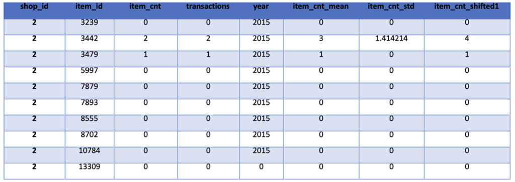
The constructor for the model then takes in the feature column name and the name of the feature being predicted. We also need to update the test data to only include the same features that we are training the model on. We show the updated test data for verification. We also show the count of rows in the test data to ensure we haven’t dropped any data.
%pyspark
from pyspark.ml.regression import RandomForestRegressor
from pyspark.ml.feature import VectorAssembler
assembler = VectorAssembler(inputCols=['shop_id', 'item_id', 'transactions', 'year', 'item_cnt_mean', 'item_cnt_std', 'item_cnt_shifted1'], outputCol="features")
transformed = assembler.transform(rf_train)
rf = RandomForestRegressor(featuresCol="features", labelCol="item_cnt_month")
rf_test = test[test_features]
%pyspark
rf_test.show(10)
%pyspark
rf_test.count()
Count of Test Data Rows: 214,200
We now train the model by calling the “fit” function with the transformed training data and display the learned feature importance. The higher the feature importance, the more influence, and impact it has on the predicted sales volume. This shows that the most influential feature is the previous month’s sales numbers followed by the average sales numbers for the item and the standard deviation of the item sales. The shop ID, item ID, and transaction count have the least influence. We then get the predictions for the validation and test sets.
%pyspark
rf_model = rf.fit(transformed)
print("Feature Importances: " + str(rf_model.featureImportances))
rf_val_pred = rf_model.transform(assembler.transform(rf_val))
predictions = rf_model.transform(assembler.transform(rf_test))

Feature Importances: (7,[0,1,2,3,4,5,6],[0.00010538864891160203,0.000521228702190239,0.03706437578651918,0.0007665815690313413,0.27629376011732415,0.22169858599322495,0.4635500791827984])
Step 5: Prediction of Future Sales
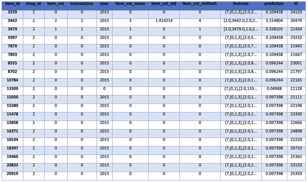
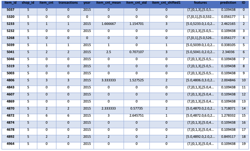
To allow us to create the expected data format for submission to the Kaggle competition, we join the test predictions with the initial ID included in the test.csv file based on the unique item_id and shop_id pair. We then display the predictions for review.
%pyspark
predictions = predictions.join(sales_test, ['item_id', 'shop_id'])
predictions.show()
To understand the accuracy of the model on the training and validation data sets, we calculate and print the root mean square error of the predictions. We will then be able to compare this to the actual results for the test data set to understand if the model is being overfitted and should be adjusted in any way.
%pyspark
rf_train_pred = rf_model.transform(transformed)
%pyspark
from pyspark.ml.evaluation import RegressionEvaluator
evaluator = RegressionEvaluator(labelCol = "item_cnt_month", predictionCol="prediction", metricName="rmse")
rmse = evaluator.evaluate(rf_train_pred)
print("Root Mean Squared Error (RMSE) on training data = %g" % rmse)
rmse_val = evaluator.evaluate(rf_val_pred)
print("Root Mean Squared Error (RMSE) on validation data = %g" % rmse_val)
Root Mean Squared Error (RMSE) on training data = 0.407676
Root Mean Squared Error (RMSE) on validation data = 0.477755
Our final steps are to prepare the results for submission to Kaggle by sorting the results by the ID and then removing all of the features to leave us with an ID and a predicted sales count. This data can then be written to disk and submitted to Kaggle.
%pyspark
predictions = predictions.orderBy("ID")
predictions.show()
%pyspark
predictedSales = predictions.select(F.col("ID"), F.col("Prediction").alias("item_cnt_month")).orderBy(F.col("ID"))
predictedSales.show()

%pyspark
predictedSales.write.parquet("s3://qubole.workshop.defloc/tmp/2019-03-26/predictions.parquet",mode="overwrite")
In the end, our model does fairly well for a simple RandomForestRegression approach to the time series analysis of sales data. Per Kaggle, we ended up with an RMSE of the test data of 1.15152.
Overall, we hope this entry helps you understand the approaches to using historical sales data to predict future sales data using the power of Qubole and PySpark.
References
Explore the references below for more information on PySpark, Zeppelin, and Random Forest Regression: