Intro
Have you ever had trouble deciding how large to make a cluster? Do you sometimes feel like you’re wasting money when a cluster isn’t being fully utilized? Or do you feel like your analysts’ time is being wasted, waiting for a query to return? At Qubole, we developed auto-scaling in order to help combat these problems.
Auto-scaling removes and adds cluster nodes depending on the workload. You simply select a minimum and a maximum number of nodes and the auto-scaling algorithm does the rest. Workloads can be unpredictable day-to-day or hour-to-hour; auto-scaling lets you sit back and not have to worry about mis-sizing a cluster. Qubole was the first Big Data platform to introduce auto-scaling back in 2012, and we have been improving it ever since.
We wanted to show that auto-scaling can help with a number of challenges, such as:
- Cluster underutilization causes wasted node hours
- Cluster overload leads to slower execution
To demonstrate the utility of auto-scaling, we decided to simulate a real customer’s workload on three clusters:
- A static cluster with 5 slave nodes
- A static cluster with 10 slave nodes
- A cluster that auto-scales between 1 and 10 slave nodes
Our analysis resulted in two key takeaways. First, the 5 node cluster was almost twice as slow as the auto-scaling cluster, but it was only incrementally cheaper. Second, the 10 node cluster was a little bit faster than the auto-scaling cluster, but it was more expensive by a third, which can really add up quickly for compute costs.
| 5 static is slower than Auto-scaling by 90% | 5 static is less expensive than Auto-scaling by 10% |
| 10 static is faster than Auto-scaling by 13% | 10 static is more expensive than Auto-scaling by 32% |
Results
| Cluster | Total Number of Node Hours | Total Runtime (in Hours) |
| 5 Static | 90* | 146 |
| 10 Static | 132 | 67 |
| 1-10 Auto-scaling | 100 | 77 |
Auto-scaling vs. 5 Nodes
The 5 node cluster took 8,757 minutes total, while the scaling cluster took only 4,644. This means that the 5 node cluster was 90% slower than the auto-scaling cluster; auto-scaling was almost twice as fast!
If we compare in terms of node hours, we can see that the auto-scaling cluster used 100 node hours, while the 5 node cluster used 90 node hours. This means that the 5 node cluster used only 10% more node hours than the auto-scaling cluster. Those 10 additional node hours buy you almost 70 hours your analyst could spend deriving essential business insights rather than waiting for a query to return.
Auto-scaling vs. 10 Nodes
The 10 node cluster took 3,999 minutes and the scaling cluster took 4,644. This means that the 10 node cluster ran about 13% faster than the auto-scaling cluster. This makes sense because the static cluster always had at least as many nodes active as the auto-scaling cluster. While 13% isn’t anything, it isn’t significant when compared to the cost-saving in terms of node hours.
If we compare the node hours, we see that the 10 static clusters used 132 node hours, while the auto-scaling cluster used only 100 node hours. This means that the 10 static clusters cost 32% more than the auto-scaling cluster. This dwarfs the 13% advantage that the static 10 node cluster has in terms of performance.
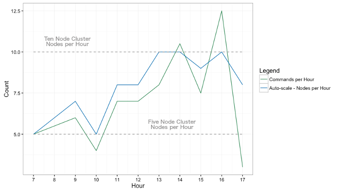
Commands per hour are plotted against the number of nodes in each hour; the commands per hour are based on a real customer’s workload
Setup
For this particular benchmark analysis, we decided to focus on the benefits of auto-scaling for data analysts (as opposed to data scientists or data engineers). Data analysts tend to issue queries from the UI and their queries tend to be highly specific. Importantly, the timing of their queries tends to be ad hoc, which compounds their unpredictability. In future benchmarks, we will look at more varied use cases with more job types and concurrency.
Commands Per Hour
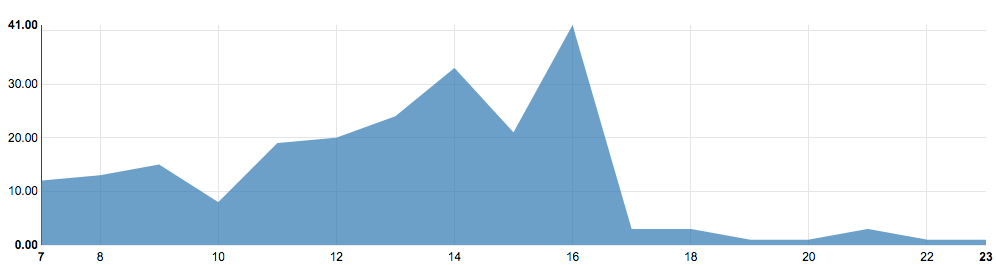
The number of commands by the hour; made using a Zeppelin notebook
We selected a typical day for a real customer cluster that ran jobs only from the Qubole’s ‘Analyze UI’ (used mostly by data analysts) and counted the number of commands in every hour (visualized in the line chart above). To improve reproducibility, we scaled down the workload by dividing the number of commands by two and rounding the result. We decided to focus on the 10 hours with the highest numbers of commands: 7 AM to 5 PM. This resulted in the following number of commands per hour:
| Hour | 7 AM | 8 AM | 9 AM | 10 AM | 11 AM | 12 PM | 1 PM | 2 PM | 3 PM | 4 PM | 5 PM |
|---|---|---|---|---|---|---|---|---|---|---|---|
| Number of Commands Run | 6 | 7 | 8 | 4 | 10 | 10 | 12 | 17 | 11 | 21 | 2 |
The number of commands per hour in this cluster varies a lot throughout the day. This high amount of variation is typical and follows the trend we would expect to see: during the workday (7 AM-5 PM) there is much more activity than during the evening, night, and early morning–there are actually no commands run between midnight and 7 AM.
This big variation in the number of commands per hour is partially explained by the difference in the number of users active in each hour. The line graph below shows how many users were active in each hour and the huge variation in how many commands each user issued. Tommen (user name obfuscated to protect customer privacy) ran just 3 queries total; Arya by contrast ran 16 queries in just one hour. These variations account for how unpredictable the load on a cluster may be at any given hour.
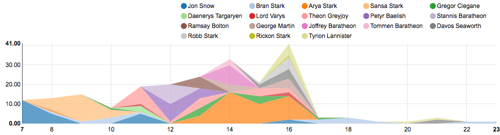
The number of commands by hour by the user; made using a Zeppelin Notebook
Query Selection
We chose TP-CDS (the standard benchmark for Big Data systems) Query 42, which typifies the query an analyst would use. Query 42 has a lot of specificities and is clearly an ad hoc query. We had to superficially modify the query to make it compatible with Spark SQL. You can find a copy of our modified query here.
We then scheduled the number of commands for each hour (6 commands for 7 AM, 7 commands for 8 AM, etc) for each one of the clusters. The queries were run concurrently and kicked off at the top of the hour.
Environment Details
The clusters had the following configurations:
- Spark version 1.6.1
- Master node type and slave node type: r3.xlarge – 4 cores, 30.5GiB mem
- Cluster auto-termination disabled*
- On-demand instances
- Default Spark configurations
- spark.executor.cores 2
- spark.executor.memory 5120M
- spark.storage.memoryFraction 0.5
Raw Results
Total Time Taken
| Hour | Number of Commands | 5 Static | 10 Static | 1-10 Auto-scaling |
| 7 AM | 6 Commands | 269 Minutes | 209 Minutes | 298 Minutes |
| 8 AM | 7 Commands | 320 Minutes | 247 Minutes | 288 Minutes |
| 9 AM | 8 Commands | 396 Minutes | 265 Minutes | 389 Minutes |
| 10 AM | 4 Commands | 152 Minutes | 118 Minutes | 193 Minutes |
| 11 AM | 10 Commands | 678 Minutes | 423 Minutes | 433 Minutes |
| 12 PM | 10 Commands | 781 Minutes | 325 Minutes | 472 Minutes |
| 1 PM | 12 Commands | 1,117 Minutes | 396 Minutes | 488 Minutes |
| 2 PM | 17 Commands | 1,977 Minutes | 608 Minutes | 709 Minutes |
| 3 PM | 11 Commands | 604 Minutes | 412 Minutes | 405 Minutes |
| 4 PM | 21 Commands | 274 Minutes | 733 Minutes | 704 Minutes |
| 5 PM | 2 Commands | 2,189 Minutes | 263 Minutes | 265 Minutes |
Node Count (excludes master node)
| Hour | 5 Static | 10 Static | 1-10 Auto-scaling |
| 7 AM | 5 Nodes | 10 Nodes | 5 Nodes |
| 8 AM | 5 Nodes | 10 Nodes | 6 Nodes |
| 9 AM | 5 Nodes | 10 Nodes | 7 Nodes |
| 10 AM | 5 Nodes | 10 Nodes | 5 Nodes |
| 11 AM | 5 Nodes | 10 Nodes | 8 Nodes |
| 12 PM | 5 Nodes | 10 Nodes | 8 Nodes |
| 1 PM | 5 Nodes | 10 Nodes | 10 Nodes |
| 2 PM | 5 Nodes | 10 Nodes | 10 Nodes |
| 3 PM | 5 Nodes | 10 Nodes | 9 Nodes |
| 4 PM | 5 Nodes | 10 Nodes | 10 Nodes |
| 5 PM | 5 Nodes | 10 Nodes | 8 Nodes |
| 6 PM | 5 Nodes | 0 Nodes | 0 Nodes |
| 7 PM | 5 Nodes | 0 Nodes | 0 Nodes |
Looking Ahead
This is the first in a series of blog posts exploring auto-scaling. For the sake of simplicity, in this benchmarking analysis, we decided to only look at the benefits of auto-scaling to data analysts using Qubole. But Qubole has a diverse range of user types, including not just analysts but data engineers and data scientists as well. In our next benchmarking, we are going to use a more diverse set of queries to capture the diversity of use cases.