Presto Optimizations for Aggregations Over Distinct Values

DISTINCT is a frequently used operator in data analytics to find the distinct values of a column in a table. It can be used along with an aggregation function, ∑(DISTINCT col) — where ∑ is an aggregate function like MIN, MAX, SUM, AVG, COUNT, etc. — to perform the aggregation over only the distinct values of a column to generate a single scalar result or a set of rows when the GROUP BY clause is used.

Executing Presto queries with the DISTINCT operation used to be slow, but over time a few optimizations have been added to Presto to speed up the execution. We will cover two such optimizations in this blog:

1. Optimizing queries with a single aggregation function aggregating over DISTINCT
2. Optimizing queries with multiple aggregations where one is aggregating on DISTINCT (contributed by Qubole)

Optimizing Queries with a Single Aggregation Function Over DISTINCT

Presto has an optimization for queries with only a single aggregation function, aggregating over DISTINCT. This optimizer is available behind the optimizer.optimize-single-distinct configuration in older versions of Presto. To understand this optimization, first, let us look at how a query with single aggregation on distinct values will execute without any optimization. Figure 1 below shows the EXPLAIN ANALYZE plan for a sample single distinct query:

SELECT
  COUNT(DISTINCT ss_customer_sk)
FROM tpcds_orc_3000.store_sales

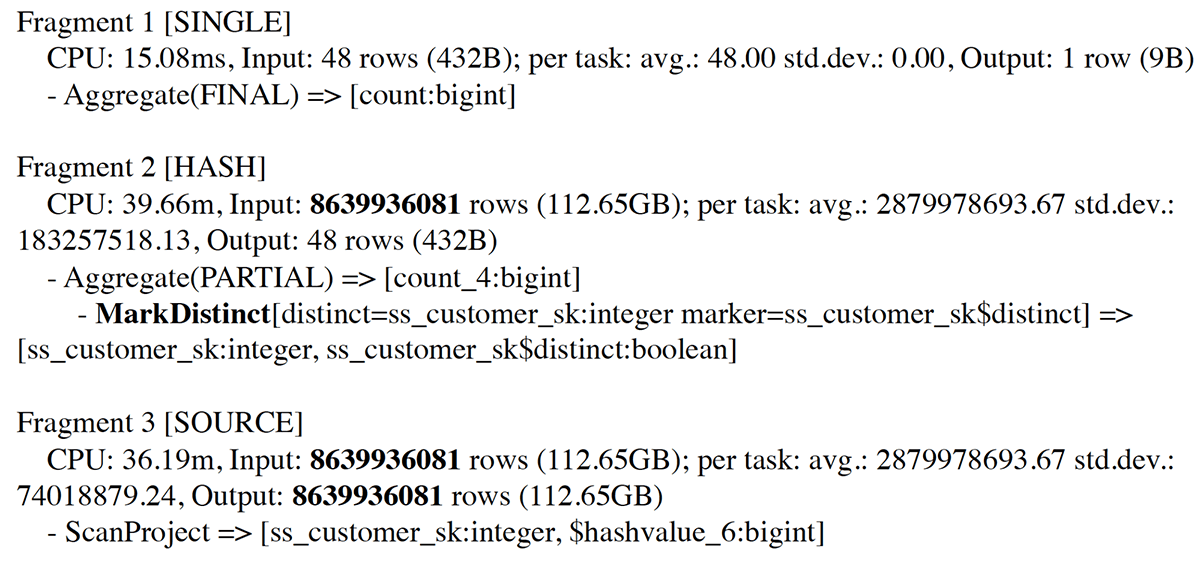Figure 1. Original Explain Analyze plan (shortened) for aggregations on distinct

As illustrated in Figure 1, after the entire data is read through the Full Table Scan in the SOURCE stage (Input=Output=8.6 billion rows), Fragment 3 sends full table data to Fragment 2, which results in a lot of network transfer. This makes the process extremely slow, especially for a data source with hundreds of millions of rows.

The Optimize-single-distinct optimizer rule in Presto brings down the amount of data that flows out from the SOURCE stage, thus decreasing the network I/O. This is achieved by partially grouping data by the distinct symbol at the SOURCE stage and then sending the data. In terms of SQL, a query like:

SELECT
  COUNT(DISTINCT ss_customer_sk)
FROM tpcds_orc_3000.store_sales

Is converted into the optimized form:

SELECT
  COUNT(*)
FROM (SELECT
  ss_customer_sk
FROM tpcds_orc_3000.store_sales
GROUP BY ss_customer_sk)

The improvement in network I/O can be seen below with the EXPLAIN ANALYZE plan of the original query with the optimization enabled:
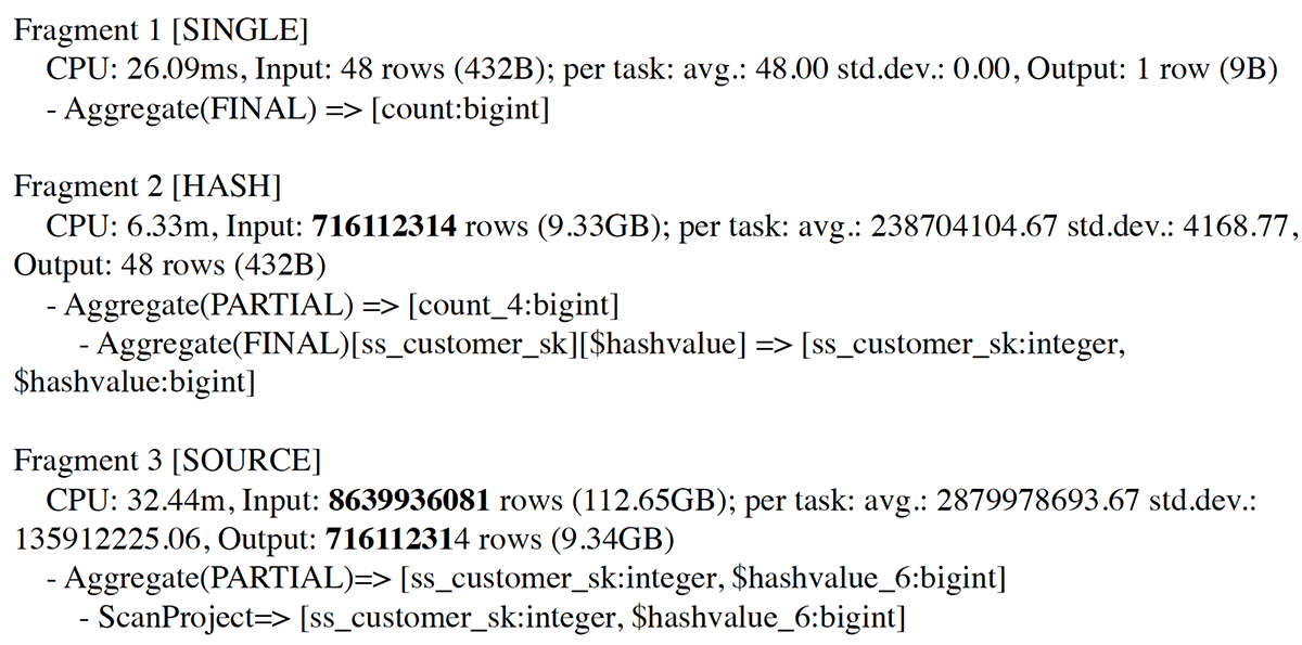
Figure 2. Optimized Explain Analyze plan (shortened) for aggregations on distinct

As shown in Figure 2, the optimizer reduces the input size of 8.6 billion rows in Fragment 3 (SOURCE stage) to an output of 716 million rows that is eventually exchanged with Fragment 2. Fragment 3 is otherwise transferred as a whole without the optimizer enabled, as explained in Figure 1, leading to faster execution (Figure 3). 

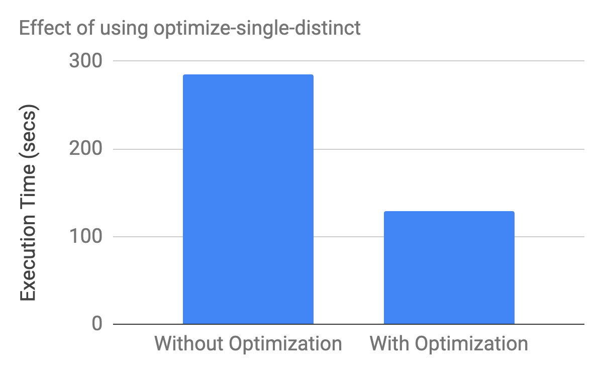
Figure 3. Executing SELECT COUNT (DISTINCT ss_customer_sk) FROM tpcds_orc_3000.store_sales, yields roughly more than 2.5x performance improvement with the optimize-single-distinct enabled.

Optimizing Queries with Multiple Aggregations Where One Is Aggregating on DISTINCT

Query performance worsens in the case of multiple aggregation functions where one of them is aggregating on DISTINCT. The optimization for single distinct optimization does not extend to such queries with multiple aggregations. For these kinds of queries, Presto has an optimization that is enabled by the optimizer.optimize-mixed-distinct-aggregations configuration. To understand this optimization, let us look at how a query with multiple aggregation functions where one is aggregating on DISTINCT will execute without any optimization. Figure 4 below shows the explained plan for a sample query:

SELECT
  ss_store_sk,
  SUM(ss_quantity),
  COUNT(DISTINCT ss_customer_sk)
FROM store_sales_100_orc
GROUP BY ss_store_sk

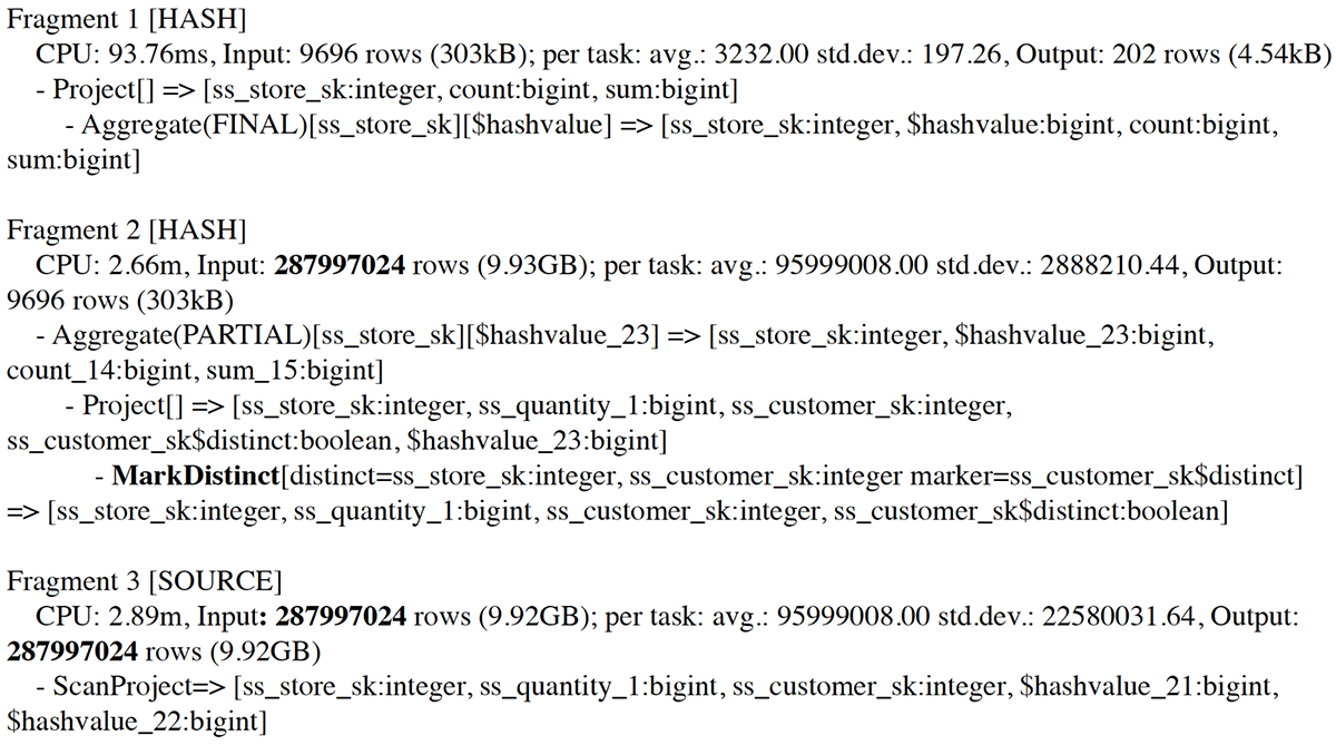
Figure 4. The limitation with multiple aggregations with a DISTINCT operator on one of the aggregations.

As illustrated in Figure 4, Fragment 3 (SOURCE stage) reads the entire data (Input = Output = 287 million rows) through a table scan and again sends the full data to Fragment 2. This causes a lot of network transfer, thereby slowing down the execution time of the query.

Multiple aggregations where one is aggregating on DISTINCT can benefit from the concept of Grouping Sets, which can make the query processing order of magnitude faster than its non-optimized version. For example,

SELECT
  COUNT(DISTINCT a) as c0,
  AVG(b) as c1
FROM table

Can be converted into its optimized form:

ELECT count(CASE groupId WHEN 1 THEN c ELSE NULL) c0,
       arbitrary(CASE groupId WHEN 0 THEN f1 ELSE NULL) c1
FROM
SELECT avg(b) f1,
       a
FROM
SELECT a,
       b
FROM table1
GROUP BY GROUPING SETS ((a), (b))
GROUP BY a, groupId

Note that unlike the optimization on single aggregation on DISTINCT explained earlier, this optimization using grouping sets cannot be manually applied by transforming the query by hand. This is because the group id used in optimized form is an internal column generated by GROUPING SET that is not available for use in the query.

The optimized form of the query is much bigger than the actual query and has more operations than the actual query, but it helps to bring down the network transfer drastically. This reduction helps to improve query performance even after a more complex execution. Figure 5 illustrates the working principle of this optimization, where the original table is expanded and then grouped efficiently, leveraging the concept of Grouping Sets. This expansion and contraction of the table happen in the SOURCE stage, which reduces the amount of data transfer across stages for subsequent aggregations.

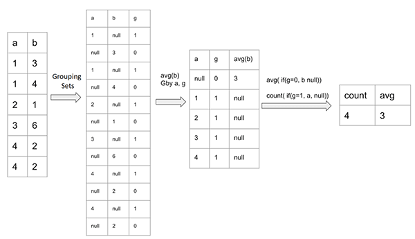
Figure 5. Working principle of OptimizeMixedDistinctAggregations for queries with multiple aggregations.

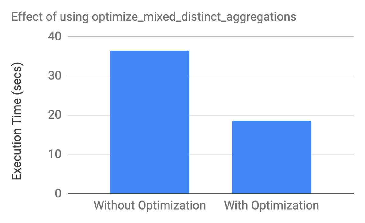
Figure 6. Executing Select ss_store_sk, sum(ss_quantity), count(DISTINCT ss_customer_sk) from store_sales_100_orc group by ss_store_sk yields roughly 2x performance improvement with the Optimize-mixed-distinct-aggregations enabled.

As shown in Figure 7, the optimizer reduces the input size of 287 million rows in Fragment 2 (SOURCE stage) to an output of 30 million rows that is eventually exchanged with Fragment 1. Fragment 1 is otherwise transferred as a whole without the optimizer enabled, as explained in Figure 4, leading to faster execution (Figure 6).

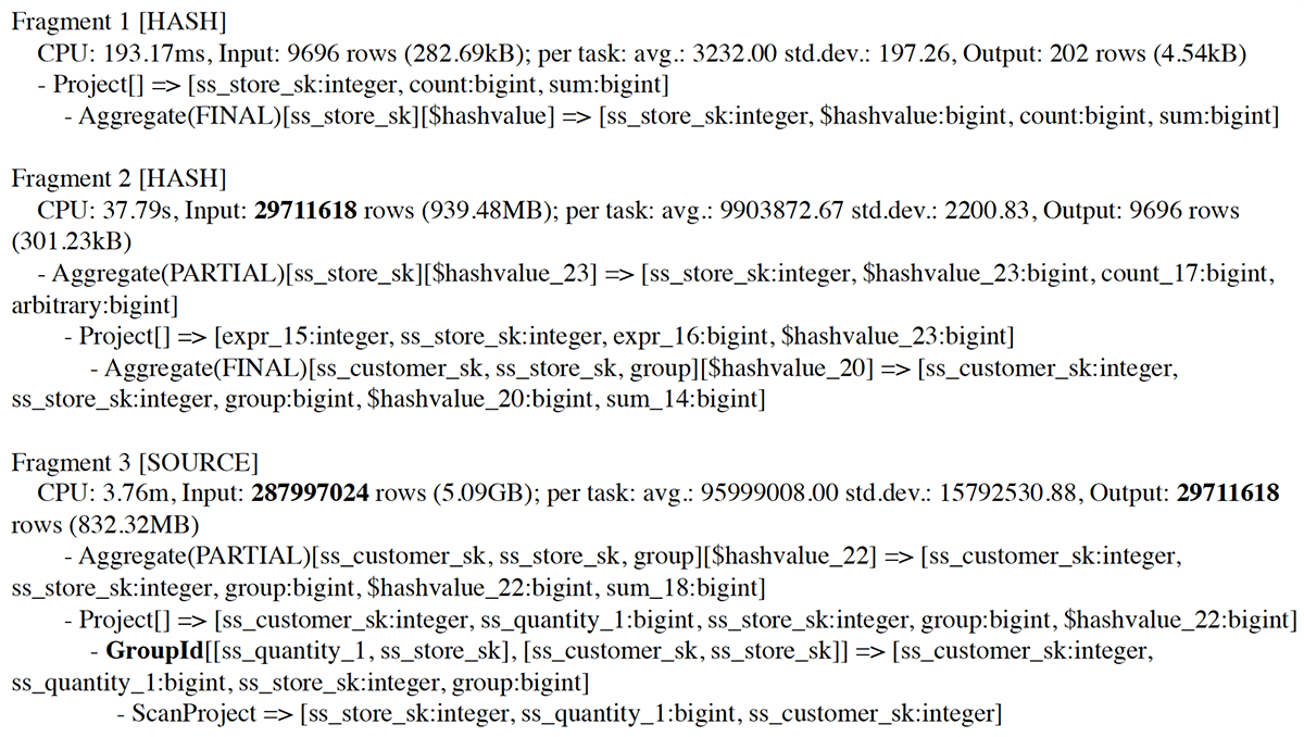
Figure 7. Optimized Explain plan (shortened) for query with multiple aggregations with DISTINCT operator on one of the aggregations:: SELECT ss_store_sk, Sum(ss_quantity), Count(DISTINCT ss_customer_sk) FROM store_sales_100_orc GROUP BY ss_store_sk

Please note, that the performance improvement depends on the cardinality of Grouping Sets in the SOURCE stage. The lower the number of groups generated by it, the better the performance is as seen in Figure 5, where there is a reduction of 287 million rows to 30 million (95 percent reduction).

Benchmark

We created a benchmark of three queries to compare the performance with and without the optimization enabled using the following tables 

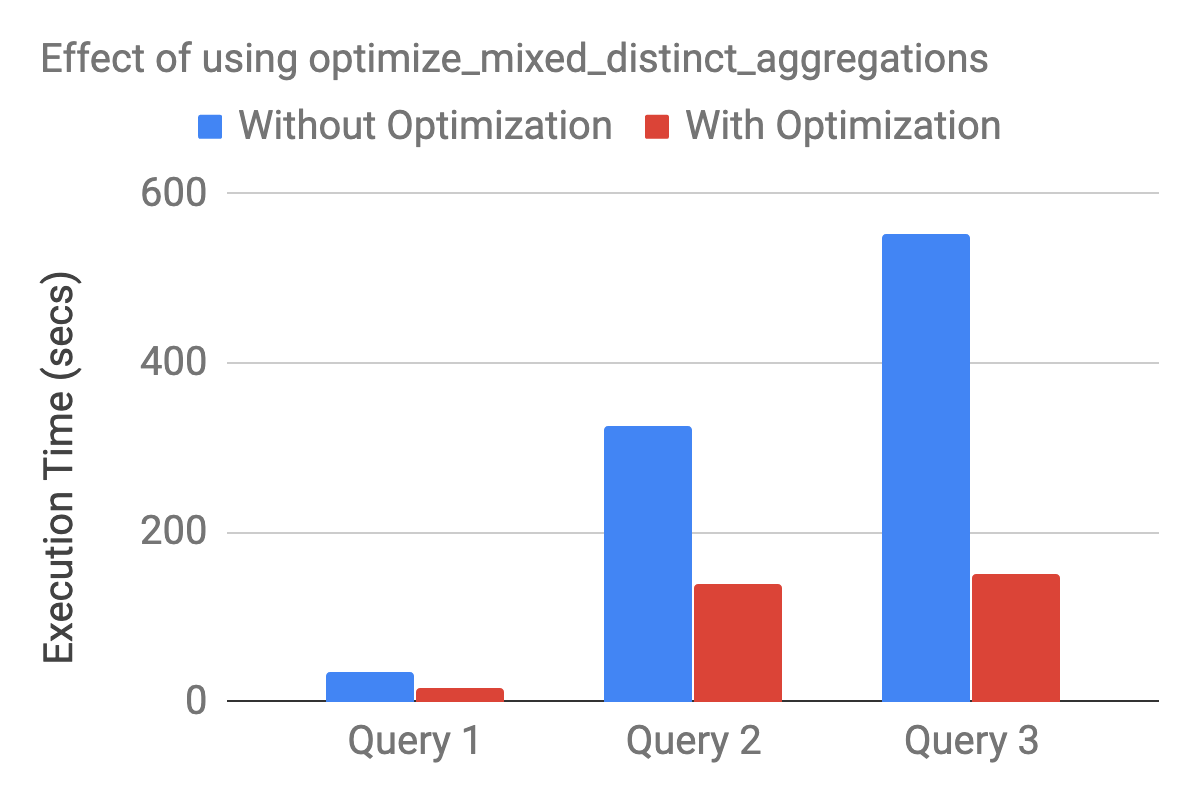
Figure 8. Optimize-mixed-distinct-aggregations yields roughly 2x-3x performance improvement on the benchmark queries.

Enabling Optimizations for DISTINCT

The optimizer.optimize-single-distinct to enable Single Distinct Aggregation Optimizer is already enabled in older versions of Presto, and in newer versions (0.208 in Qubole) the configuration has been deprecated and the queries always get converted into the optimized form.

To enable optimization for queries having multiple aggregations where one of them is aggregating on DISTINCT, the following configuration goes into config.properties:

optimizer.optimize-mixed-distinct-aggregations=true.

This configuration can be configured in Qubole under Presto Settings on the Edit Cluster page:

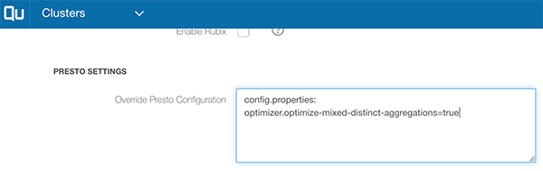
This optimization can also be enabled on a per-query basis by using
optimize_mixed_distinct_aggregations session property as follows:

SET SESSION optimize_mixed_distinct_aggregations=true;

Ongoing Works

Currently, optimize-mixed-distinct-aggregations optimizes a query if there is only one aggregation on the DISTINCT operation. There is work going on now to extend this concept of Grouping Sets for queries with multiple aggregation functions aggregating over a DISTINCT operator. There has been a recent contribution to OSS in the same context, which shows an improvement of 2.5x to 3x using Grouping Sets on multiple distinct aggregation queries.