Drug discovery is the process of identifying molecular compounds which are likely to become the active ingredient in prescription medicine. At a high level, it works by taking a set of candidate compounds (either synthetic or naturally derived) and evaluating their chemical reactions with (an often cloned) molecule which is largely correlated with a particular disease [1]. Machine learning, and deep learning in particular, have been highly successful in predicting the chemical reactions between candidate compounds and target molecules [2, 3, 4]. These models have enabled biomedical engineers to rapidly iterate on the design of new synthetic compounds by querying a trained deep neural network to estimate how a candidate compound would interact with a target molecule. This enables the largest pharmaceutical companies, such as Merck, to significantly reduce their drug discovery costs.
Applications of machine learning such as these typically require a cluster of GPU machines to perform parallel model training or parallel model selection, or both. Cloud providers minimize the capital expenses otherwise incurred on the initial deployment of such clusters. Qubole Data Service (QDS) minimizes the time and operating expenses otherwise incurred on maintaining and updating such infrastructure. This demonstration, therefore, utilizes the framework developed in my blog post on distributed deep learning within QDS [5].
The Goal: Drug Discovery Using Deep Learning On The Merck Molecular Activity Dataset
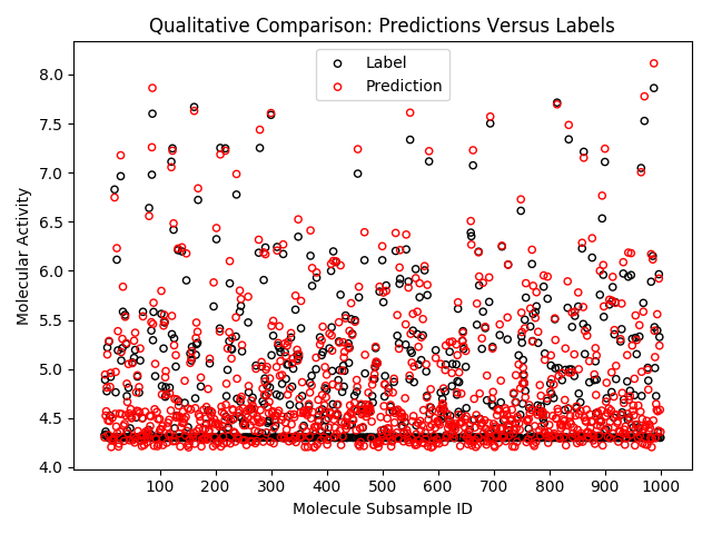
Upon completion of this blog post, an enterprising data scientist should have trained at least one deep neural network to predict molecular activity on the Merck dataset. Within a Qubole notebook [7], you will cross validate your DNNs using the Spark ML Pipeline interface [6], while maintaining the big data best practices implemented in QDS [8]. The resulting prediction quality will be reported as an R2 score [9], as well as visually inspected with a scatter plot overlaying the model outputs with the corresponding labels.
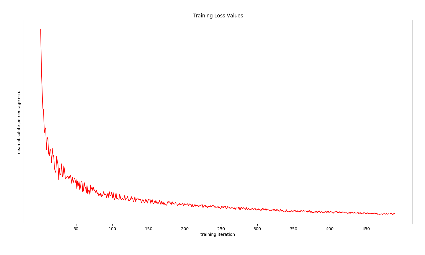
The convergence of training will also be verified by plotting the loss function of the best cross validated model, as it is retrained on training data plus holdout data. Important to note that the loss function decreases towards a non-unique minima. There may be better minima in the cost function topology.
R2 score on holdout validation data may be estimated using the following example code. Note this quantitative metric lacks the ability to describe the quality of the trained model (eg., favoring predictions around 4.3 as seen in the labels, but overestimating molecular activity on aggregate).
##
# `cv_model` and `evaluator` both defined in example code to cross validate
##
df_predictions = cv_model.transform(df_holdout)
r2_score = evaluator.evaluate(df_predictions)
print(r2_score)
0.915
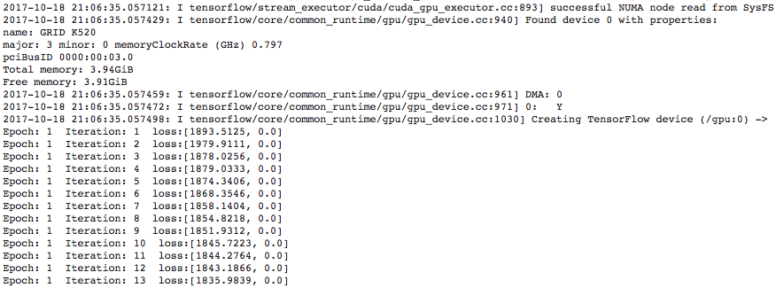
Last but not least, GPU utilization and decreasing loss function values may be viewed during training by inspecting the Spark executor log file output. Instructions for navigating to these logs can be found at the last entry of this blog.
Example Code To Cross Validate Your Drug Discovery Models
Working within the framework laid out in my blog post on distributed deep learning within QDS [5], you must specific your input dataset and which columns to rename, then exclude from the training features. This example uses the ACT01 dataset from the Merck molecular activity challenge [10]
base_dir = "//fully/qualified/path/to/root/folder/of/dataset/"

excluded_columns = ('MOLECULE', 'label')
columns_renamed = (('Act', 'label'), )

train_set = "ACT01_training.csv"
test_set = "ACT01_testing.csv"

num_workers = 50
The base directory will be some persistent cloud storage, such as Amazon S3 or Azure Blobs, and the number of workers must be identical to the number of Spark executors currently running in your cluster. Next step is to ingest DataFrames from the CSV data, and to define the parameter grid over which you will cross validate your drug discovery models. Here is a reasonable grid with which to begin on the ACT01 dataset
df_train = process_csv(base_dir + train_set,
                       columns_renamed=columns_renamed,
                       excluded_columns=excluded_columns,
                       num_workers=num_workers)
df_test = process_csv(base_dir + test_set,
                      columns_renamed=columns_renamed,
                      excluded_columns=excluded_columns,
                      num_workers=num_workers)

input_dim = 9491

param_grid = tuning.ParamGridBuilder() \
                   .baseOn(['regularizer', regularizers.l1_l2]) \
                   .addGrid('activations', [['tanh', 'relu']]) \
                   .addGrid('initializers', [['glorot_normal',
                                              'glorot_uniform']]) \
                   .addGrid('layer_dims', [[input_dim, 2000, 300, 1]]) \
                   .addGrid('metrics', [['mae']]) \
                   .baseOn(['learning_rate', 1e-2]) \
                   .baseOn(['reg_strength', 1e-2]) \
                   .baseOn(['reg_decay', 0.25]) \
                   .baseOn(['lr_decay', 0.90]) \
                   .addGrid('dropout_rate', [0.20, 0.35, 0.50, 0.65, 0.80]) \
                   .addGrid('loss', ['mse', 'msle']) \
                   .build()
Lastly, you need to define an estimator and an evaluation metric against which it will be cross validated. All tuning will be done with the Spark ML pipelines, leveraging the framework in [5].
estimator = DistKeras(trainers.ADAG,
                      {'batch_size': 64,
                       'communication_window': 3,
                       'num_epoch': 5,
                       'num_workers': num_workers},
                      **param_grid[0])

evaluator = evaluation.RegressionEvaluator(metricName='r2')

cv_estimator = tuning.CrossValidator(estimator=estimator,
                                     estimatorParamMaps=param_grid,
                                     evaluator=evaluator,
                                     numFolds=4)
cv_model = cv_estimator.fit(df_train)
Example Code To Visualize Prediction Quality And Verify Decreasing Training Loss
Spark ML Pipelines API enables us to compute R2 scores [9], to run a trained model and obtain predictions, as well as providing us with a reference to the best Dist-Keras model from our cross validation above. The code below demonstrates how to leverage all of these
##
# equivalently:
#   dist_keras_model = cv_model.bestModel
#   df_predictions = dist_keras_model.transform(df_holdout)
##
df_predictions = cv_model.transform(df_holdout)
df_predictions = df_predictions.select('label', 'prediction').toPandas()
yt = df_predictions['label'].as_matrix()
yp = df_predictions['prediction'].as_matrix()
Note the selection of only label and prediction column, prior to collecting into a local Pandas DataFrame. Random sampling 1K labels and predictions yields the qualitative comparison exemplified in the goals section of this demonstration.
fig = plt.figure()

idx = np.random.randint(df_predictions.count(), size=1000)
nx = np.arange(1000) + 1

axa = fig.add_subplot(121)
_ = axa.scatter(nx, yt[idx], s=20, facecolors='none', edgecolors='k')
_ = axa.scatter(nx, yp[idx], s=20, facecolors='none', edgecolors='r')
_ = axa.set_title('Qualitative Comparison: Predictions Versus Labels')
_ = axa.set_xticks([j for j in nx if not j % 100])
_ = axa.set_xticklabels([str(j) for j in nx if not j % 100])
_ = axa.set_xlabel('Molecule Subsample ID')
_ = axa.set_ylabel('Molecular Activity')
_ = axa.legend(('Label', 'Prediction'))
Dist-Keras provides us with the history of loss function values during training [11], as well as giving us access to the native Keras model trained in a data parallel fashion. The latter provides a function which outputs the model layout in a format which is easy to plot [12]. The code below leverages these features to complete our intended goal for this demonstration.
loss_and_metrics = dist_keras._trainer.get_averaged_history()
x = np.arange(loss_and_metrics.shape[0]) + 1
y = np.array(map(itemgetter(0), loss_and_metrics))

axb = fig.add_subplot(122)
_ = axb.plot(x, y, 'r-')
_ = axb.set_title('Training Loss Values')
_ = axb.set_xticks([j for j in x if not j % 50])
_ = axb.set_xticklabels([str(j) for j in x if not j % 50])
_ = axb.set_xlabel('training iteration')
_ = axb.set_ylabel('mean absolute percentage error')

fig.tight_layout()
show(fig)

##
# plot structure of best cross validated model to file
##
keras_model = dist_keras_model._keras_model
utils.plot_model(keras_model, to_file='drug_discovery_cv_model.png')
Viewing Logs During Model Training
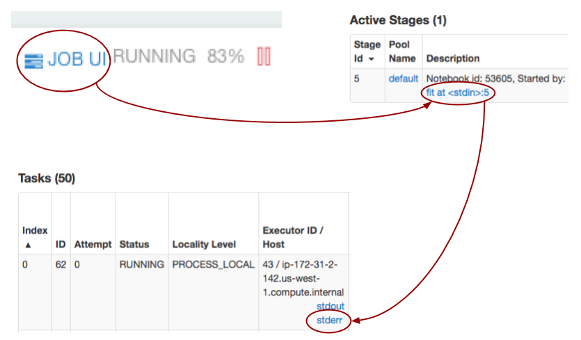
Within your Qubole notebook [7], you have the ability to view Spark executor logs [13] while your model is training. To view these logs in an overlaid frame, simply click on `Job UI` and follow the dark red arrows in the diagram below for subsequent clicks. Clicking on `stderr` will result in a log file similar to that in the goals section of this post.
About The Author
Horia Margarit is a career data scientist with industry experience in machine learning for digital media, consumer search, cloud infrastructure, life sciences, and consumer finance industry verticals [14]. His expertise is in modeling and optimization on internet scale datasets, specifically leveraging distributed deep learning among other techniques. He earned dual Bachelors degrees in Cognitive and Computer Science from UC Berkeley, and a Master’s degree in Statistics from Stanford University.
References
- Wikipedia: Drug Discovery
- Team ‘.’ takes 3rd in the Merck Challenge
- Team DataRobot: Merck 2nd place Interview
- Deep Learning How I Did It: Merck 1st place interview
- Distributed Deep Learning with Keras on Apache Spark
- Spark ML Pipelines
- Introduction To Qubole Notebooks
- The Cloud Advantage: Decoupling Storage And Compute
- Wikipedia: R2 Scores
- Merck Molecular Activity Challenge
- Dist-Keras: History Of Loss Function Values
- Wikipedia: DOT (graph description language)
- Apache Spark: Monitoring And Instrumentation
- Author’s LinkedIn Profile