For many data scientists and statisticians, R is their tool of choice. It provides many useful abstractions, is easy to script in, and has tons of useful packages. And for users of R, RStudio is the go-to interface for writing and editing code. RStudio allows users to quickly iterate on their scripts and create shareable notebooks for collaboration and reproducibility.
Unfortunately, R users who wanted to use Apache Spark to quickly analyze large datasets have historically been unable to do so in their favorite environment. But now, with Qubole and the Livy server, R users can connect the RStudio on their laptop directly to their Spark cluster and analyze terabytes of data with their favorite language.
With the Livy integration, data scientists can use packages like dplyr and ggplot2 to manipulate and visualize their data. They can also use Spark’s machine learning library spark.ml to train models like linear regressions and random forests. Developing a machine learning workflow with RStudio and sparklyr has the ease of development on your laptop, with the computational power of a computing cluster.
Setting Up the Connection to Your Spark Cluster
Connecting your Spark cluster using Livy is incredibly easy. First we set up the Livy server on the Spark cluster, then proceed to connect to it from our locally running RStudio.
To set up the Livy server, you need to modify the node bootstrap of the Spark cluster you wish to connect to. You can either create a new Spark cluster for this purpose or modify an existing one, but in either case you can see the location of your node bootstrap script in the “Configuration” section of the “Edit Cluster” page. Modify your bootstrap file to include the following snippet of code:
source /usr/lib/hustler/bin/qubole-bash-lib.sh

is_master=`nodeinfo is_master`

if [[ "$is_master" == "1" ]]; then

cd /media/ephemeral0
mkdir livy
cd livy
wget https://archive.cloudera.com/beta/livy/livy-server-0.3.0.zip
unzip livy-server-0.3.0.zip
export SPARK_HOME=/usr/lib/spark
export HADOOP_CONF_DIR=/etc/hadoop/conf
cd livy-server-0.3.0
mkdir logs

echo livy.spark.master=yarn >> conf/livy.conf
echo livy.spark.deployMode=client >> conf/livy.conf
echo livy.repl.enableHiveContext=true >> conf/livy.conf

nohup ./bin/livy-server > ./logs/livy.out 2> ./logs/livy.err < /dev/null &

fi
Once this script is included in your node bootstrap file, start or restart your cluster and make sure it’s up before proceeding to the next step.
Before connecting to the Livy server, you’ll need to make sure that sparklyr is installed on your machine. If you haven’t already, run install.packages(sparklyr) from the RStudio console. Then modify and run the following script:
library(sparklyr)
custom_headers <- list(`X-AUTH-TOKEN`="<API_TOKEN>")
sconfig <- spark_config()
sconfig$spark.qubole.max.executors <- 10
cfg <- livy_config(config = sconfig, "custom_headers" = custom_headers)
sc <- spark_connect(master = "https://<ENVIRONMENT>.qubole.com/livy-spark-<CLUSTER_ID>", method = "livy", config = cfg)
Replace <API_TOKEN> with your API token, <ENVIRONMENT> with your subdomain (us, api, etc), and <CLUSTER_ID> with the ID of the Spark cluster which is running the Livy server.
Voila! The connection is set up, and now we’re ready to run some analysis.
Predicting Telecom Customer Churn Using Logistic Regression
In this example, we are going to be analyzing the telecom customer churn dataset open sourced by IBM. The data will require a bit of cleaning, after which we will do some light data exploration with ggplot2, and build our logistic regression model with the binary value “churned” (representing whether or not a customer has churned).
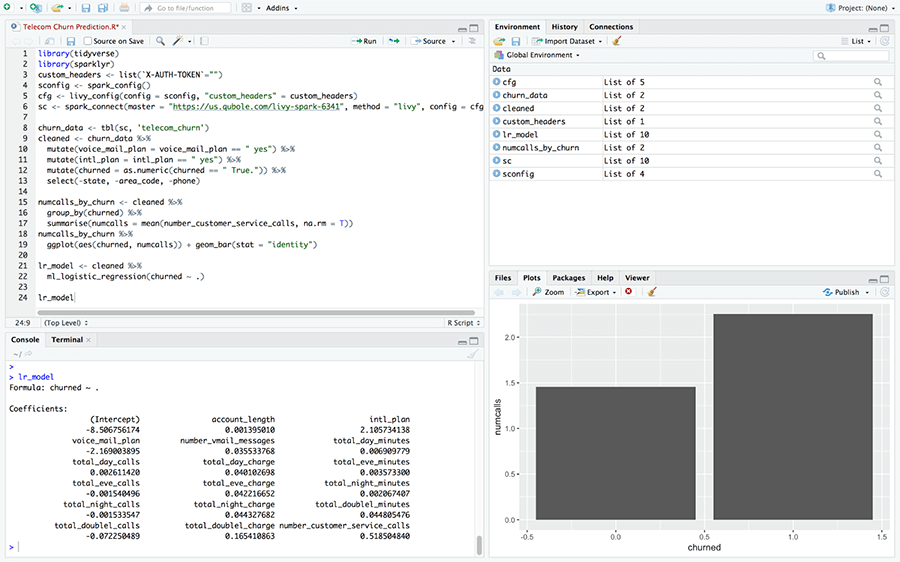
The first step is connecting our RStudio instance to our cluster. You can follow the instructions above to make the connection. Since our data is setting in a Hive metastore in the Qubole account, we need to bring the data into our Spark context. To do this, we simply run:
library(tidyverse) #required for `tbl`; also contains dplyr and ggplot2 which will be used later
churn_data <- tbl(sc, 'telecom_churn')
Now that our data is available in our Spark context, let’s use dplyr to clean the data. Some of the binary categorical variables (voice_mail_plan, intl_plan, and our response variable churned) come to us as strings; these need to be converted into boolean values in order to be analyzed later. For the sake of simplicity, let’s also remove the categorical variables with multiple categories (state, area_code, and phone). We can use dplyr to do all of these things like so:
cleaned <- churn_data %>%
  mutate(voice_mail_plan = voice_mail_plan == " yes") %>%
  mutate(intl_plan = intl_plan == " yes") %>%
  mutate(churned = as.numeric(churned == " True.")) %>%
  select(-state, -area_code, -phone)
One variable that I would expect to be highly correlated with whether or not a customer has churned is the number of calls they make. To test this theory we could use a measure of correlation, but for our cursory examination (and to highlight the ability to use ggplot2 with the RStudio integration) let’s visualize this correlation with a bar chart. First we are going to use dplyr to find the mean number of calls in both categories (customers who have churned and customers who haven’t) and then use ggplot2 to output the visualization.
numcalls_by_churn <- cleaned %>%
  group_by(churned) %>%
  summarise(numcalls = mean(number_customer_service_calls, na.rm = T))
numcalls_by_churn %>%
  ggplot(aes(churned, numcalls)) + geom_bar(stat = "identity")
Which results in:
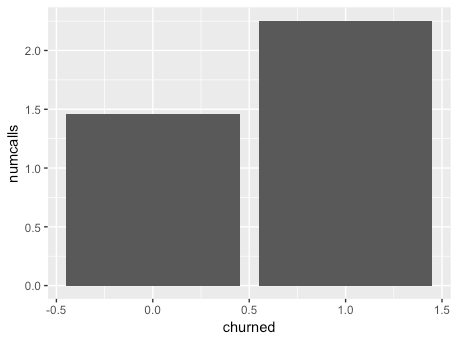
As we can see, there is indeed a correlation between the number of calls and the churned variable, which indicates that it will likely be a good predictor of whether or not a customer has churned.
Once we’ve conducted some exploratory data analysis, we can use spark.ml’s logistic regression to train the model on the data:
lr_model <- cleaned %>%
  ml_logistic_regression(churned ~ .)
Once the model is finished training, we can take a look at the coefficients by calling the model object:
> lr_model
Formula: churned ~ .

Coefficients:
                  (Intercept)                account_length
                 -8.380670181                   0.002248411
                    intl_plan               voice_mail_plan
                  2.036051147                  -2.095822560
        number_vmail_messages             total_day_minutes
                  0.035699797                   0.007006018
              total_day_calls              total_day_charge
                  0.001830694                   0.040596042
            total_eve_minutes               total_eve_calls
                  0.003582273                  -0.001591671
             total_eve_charge           total_night_minutes
                  0.043509584                   0.001769325
            total_night_calls            total_night_charge
                 -0.001444300                   0.040069531
        total_doublel_minutes           total_doublel_calls
                  0.045861092                  -0.084732775
         total_doublel_charge number_customer_service_calls
                  0.158694744                   0.515739869
From here we have lots of options: we can evaluate the performance of this model, evaluate other models, or even look for new data to contribute to the existing dataset.
Conclusion
Spark is a powerful engine for data scientists wishing to analyze vast amounts of data, and RStudio is a popular IDE among R users. With the Livy connector, we can utilize the power of Spark with the convenience of RStudio.
To see how you can use the Livy server to connect a Qubole Spark cluster with a Jupyter notebook, check out our blog post on the topic. To learn more about about the Livy project, check out the Apache Livy community page.
If you are interested in testing RStudio with Qubole Spark, please reach out to us at [email protected]. Sign-up for a free trial on Qubole.